Model Buidling Misc.

Mixed

# numerical calculation & data frames
import numpy as np
import pandas as pd

# visualization
import matplotlib.pyplot as plt
import seaborn as sns
import seaborn.objects as so

# statistics
import statsmodels.api as sm
import statsmodels.formula.api as smf

# pandas options
pd.set_option('mode.copy_on_write', True)  # pandas 2.0
pd.options.display.float_format = '{:.2f}'.format  # pd.reset_option('display.float_format')
pd.options.display.max_rows = 7  # max number of rows to display

# NumPy options
np.set_printoptions(precision = 2, suppress=True)  # suppress scientific notation

# For high resolution display
import matplotlib_inline
matplotlib_inline.backend_inline.set_matplotlib_formats("retina")

bikeshare = pd.read_csv("../data/hour.csv")
bikeshare_daily = pd.read_csv("../data/day.csv")


def clean_data(df):
    df.rename({"dteday": "date", "cnt": "count"}, axis=1, inplace=True)

    df = df.assign(
        date=lambda x: pd.to_datetime(x["date"]),  # datetime type으로 변환
        year=lambda x: x["date"].dt.year.astype(str),  # year 추출
        day=lambda x: x["date"].dt.day_of_year,  # day of the year 추출
        month=lambda x: x["date"].dt.month_name().str[:3],  # month 추출
        wday=lambda x: x["date"].dt.day_name().str[:3],  # 요일 추출
    )

    df["season"] = (
        df["season"]
        .map({1: "winter", 2: "spring", 3: "summer", 4: "fall"})  # season을 문자열로 변환
        .astype("category")  # category type으로 변환
        .cat.set_categories(
            ["winter", "spring", "summer", "fall"], ordered=True
        )  # 순서를 지정
    )
    return df


bikes = clean_data(bikeshare)
bikes_daily = clean_data(bikeshare_daily)

bikes_daily.head(3)

   instant       date  season  yr  mnth  holiday  weekday  workingday  \
0        1 2011-01-01  winter   0     1        0        6           0   
1        2 2011-01-02  winter   0     1        0        0           0   
2        3 2011-01-03  winter   0     1        0        1           1   

   weathersit  temp  atemp  hum  windspeed  casual  registered  count  year  \
0           2  0.34   0.36 0.81       0.16     331         654    985  2011   
1           2  0.36   0.35 0.70       0.25     131         670    801  2011   
2           1  0.20   0.19 0.44       0.25     120        1229   1349  2011   

   day month wday  
0    1   Jan  Sat  
1    2   Jan  Sun  
2    3   Jan  Mon  

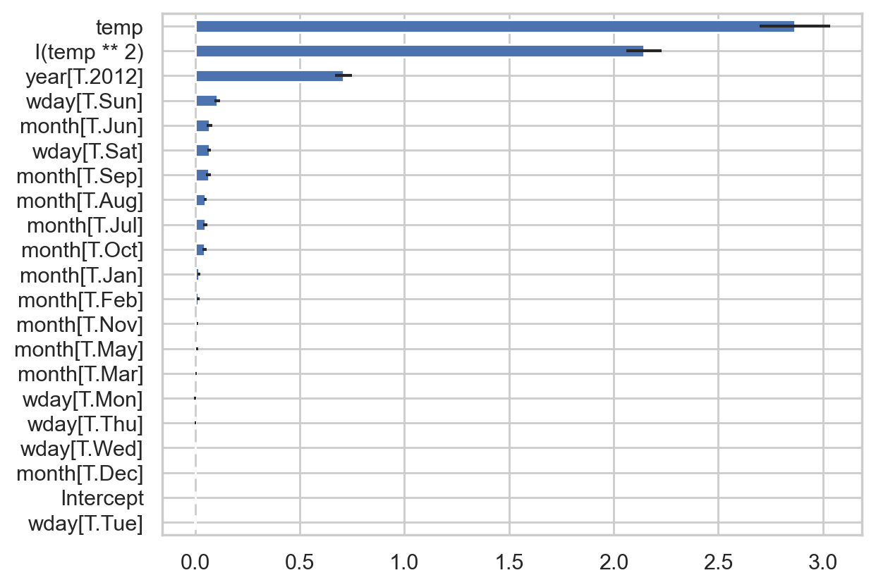
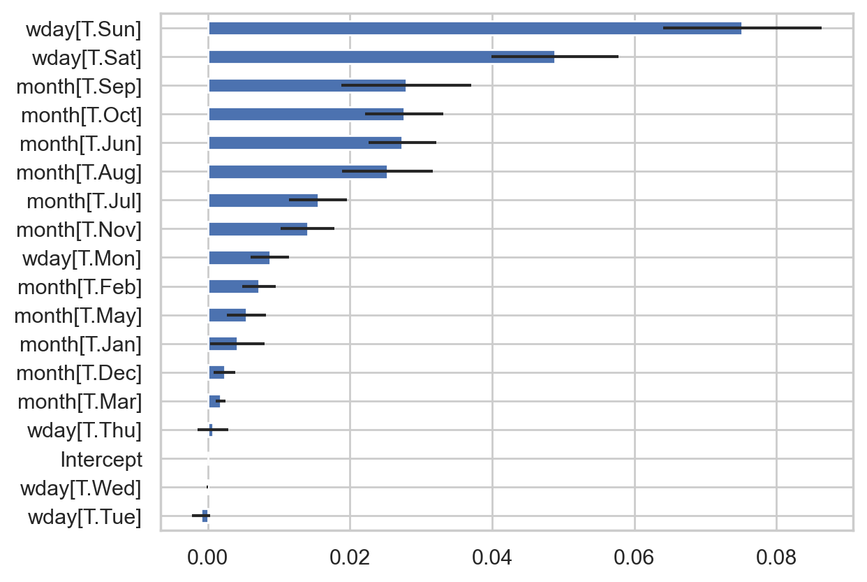
변수의 상대적 중요도

다양한 방식이 제안되어 있고 각각 한계가 있음. 예를 들어,

• 선형모형의 경우 표준화된 회귀계수(또는 T value), 부분 상관계수(partial, semi-partial correlation), 위계적 모형의 비교
• Sensitivity analysis; SALib
• Permutation importance; scikit-learn의 permutation_importance
• Tree 기반 feature importance; interpretML
• SHAP value

위계적 모형의 비교

import statsmodels.formula.api as smf

mod_r_year = smf.ols("registered ~ year", data=bikes_daily).fit()
mod_r_temp = smf.ols("registered ~ year + temp + I(temp**2)", data=bikes_daily).fit()
mod_r_month = smf.ols("registered ~ year + temp + I(temp**2) + month", data=bikes_daily).fit()
mod_r_wday = smf.ols("registered ~ year + temp + I(temp**2) + month + wday", data=bikes_daily).fit()

print(
    f" year: {mod_r_year.rsquared:.3f}\n",
    f"year + temperature: {mod_r_temp.rsquared:.3f}\n",
    f"year + temperature + months: {mod_r_month.rsquared:.3f}\n",
    f"year + temperature + months + days of the week: {mod_r_wday.rsquared:.3f}",
)

 year: 0.353
 year + temperature: 0.653
 year + temperature + months: 0.686
 year + temperature + months + days of the week: 0.757

T value / 표준화된 회귀계수

print(mod_r_wday.summary())

                            OLS Regression Results                            
==============================================================================
Dep. Variable:             registered   R-squared:                       0.757
Model:                            OLS   Adj. R-squared:                  0.750
Method:                 Least Squares   F-statistic:                     110.6
Date:                Mon, 09 Jun 2025   Prob (F-statistic):          1.66e-202
Time:                        03:42:48   Log-Likelihood:                -5894.3
No. Observations:                 731   AIC:                         1.183e+04
Df Residuals:                     710   BIC:                         1.193e+04
Df Model:                          20                                         
Covariance Type:            nonrobust                                         
================================================================================
                   coef    std err          t      P>|t|      [0.025      0.975]
--------------------------------------------------------------------------------
Intercept      -74.2636    343.767     -0.216      0.829    -749.185     600.658
year[T.2012]  1777.6982     58.315     30.484      0.000    1663.208    1892.189
month[T.Aug]   777.0600    185.742      4.184      0.000     412.390    1141.730
month[T.Dec]   113.2666    153.852      0.736      0.462    -188.793     415.326
month[T.Feb]  -438.5490    162.694     -2.696      0.007    -757.968    -119.130
month[T.Jan]  -433.1165    180.380     -2.401      0.017    -787.258     -78.975
month[T.Jul]   710.4538    212.142      3.349      0.001     293.953    1126.954
month[T.Jun]   829.2689    177.396      4.675      0.000     480.986    1177.552
month[T.Mar]  -245.4253    145.140     -1.691      0.091    -530.381      39.530
month[T.May]   420.7856    151.166      2.784      0.006     124.000     717.571
month[T.Nov]   446.4927    148.101      3.015      0.003     155.725     737.260
month[T.Oct]   716.5870    141.358      5.069      0.000     439.057     994.117
month[T.Sep]   876.4995    156.341      5.606      0.000     569.554    1183.445
wday[T.Mon]   -270.8906    107.946     -2.509      0.012    -482.823     -58.958
wday[T.Sat]   -794.1801    107.955     -7.357      0.000   -1006.129    -582.231
wday[T.Sun]  -1012.2886    107.987     -9.374      0.000   -1224.300    -800.277
wday[T.Thu]    122.9289    108.255      1.136      0.257     -89.609     335.467
wday[T.Tue]     -9.2864    108.269     -0.086      0.932    -221.851     203.278
wday[T.Wed]     32.8857    108.244      0.304      0.761    -179.630     245.402
temp          1.019e+04   1268.580      8.034      0.000    7701.355    1.27e+04
I(temp ** 2) -8061.8141   1317.345     -6.120      0.000   -1.06e+04   -5475.456
==============================================================================
Omnibus:                      255.792   Durbin-Watson:                   0.990
Prob(Omnibus):                  0.000   Jarque-Bera (JB):             1060.594
Skew:                          -1.584   Prob(JB):                    4.95e-231
Kurtosis:                       7.979   Cond. No.                         86.1
==============================================================================

Notes:
[1] Standard Errors assume that the covariance matrix of the errors is correctly specified.

Permutation importance

from sklearn.model_selection import train_test_split
from sklearn.linear_model import LinearRegression

from patsy import dmatrices
y, X = dmatrices("registered ~ year + temp + I(temp**2) + month + wday", data=bikes_daily, return_type="dataframe")

X_train, X_test, y_train, y_test = train_test_split(X, y, random_state=123, test_size=0.5)

lr = LinearRegression(fit_intercept=False)
lr.fit(X_train, y_train)

LinearRegression(fit_intercept=False)

In a Jupyter environment, please rerun this cell to show the HTML representation or trust the notebook.
On GitHub, the HTML representation is unable to render, please try loading this page with nbviewer.org.

from sklearn.inspection import permutation_importance

imp_permu = permutation_importance(lr, X_test, y_test, n_repeats=30, scoring="r2")  # default: R-squared

imp_permu_df2 = pd.DataFrame({"mean": imp_permu.importances_mean, "std": imp_permu.importances_std}, index=X.columns)

# plot imp_permu_df2 with error bars
sns.set_theme(style="whitegrid")
imp_permu_df2["mean"].sort_values().plot(kind="barh", xerr=imp_permu_df2["std"]);

imp_permu_df2.query("mean < 0.2")["mean"].sort_values().plot(kind="barh", xerr=imp_permu_df2["std"]);

ML 모형을 이용한 fitted lines

# 2012년 데이터만 이용
bikes_daily_2012 = bikes_daily.query('year == "2012"')

Spline Fits

B-spline을 이용한 모형

from sklearn.preprocessing import SplineTransformer
from sklearn.linear_model import LinearRegression
from sklearn.pipeline import make_pipeline

def spline_df(df, x, y, n_knots=10, **kwargs):
    """
    Build a dataframe of Spline regression.
    """

    df.dropna(subset=[x, y], inplace=True)
    X_, y_ = df[[x]].values, df[y].values

    B_basis = SplineTransformer(n_knots=n_knots)
    lr = LinearRegression()
    spline = make_pipeline(B_basis, lr).fit(X_, y_)

    # make a grid for prediction
    XX = np.linspace(df[x].min(), df[x].max(), 100).reshape(-1, 1)
    yy = spline.predict(XX)

    return pd.DataFrame({"x_ax": XX[:, 0], "y_ax": yy})

spline_fitted = spline_df(bikes_daily_2012, x="temp", y="registered", n_knots=8)

(
    so.Plot(bikes_daily_2012, x='temp', y='registered')
    .add(so.Dots(color=".6"))
    .add(so.Line(), so.PolyFit(2))
    .add(so.Line(color="darkorange"), x=spline_fitted["x_ax"], y=spline_fitted["y_ax"])
)

Generalized Additive Model (GAM)

참고 pyGAM
2025/5/12 scipy 1.13.1 (python 3.12)

from pygam import LinearGAM, s

def pspline_df(df, x, y, width=0.90, lam=0, **kwargs):
    """
    Build a dataframe of penalized spline regression.
    """

    df.dropna(subset=[x, y], inplace=True)
    X_, y_ = df[[x]], df[y]
    gam = LinearGAM(s(0, lam=lam, **kwargs)).fit(X_, y_)  # spline regression

    # make a grid for prediction
    XX = gam.generate_X_grid(term=0)
    yy = gam.predict(XX)
    yy_se = gam.prediction_intervals(XX, width=width)  # 90% prediction interval

    return pd.DataFrame(
        {"x_ax": XX[:, 0], "y_ax": yy, "ymin": yy_se[:, 0], "ymax": yy_se[:, 1]}
    )

psplines = pspline_df(bikes_daily_2012, x="temp", y="registered", n_splines=20, lam=5)

(
    so.Plot(bikes_daily_2012, x='temp', y='registered')
    .add(so.Dots(color=".6"))
    .add(so.Line(), so.PolyFit(5))
    .add(so.Line(color="darkorange"), x=psplines["x_ax"], y=psplines["y_ax"])  # penallized spline fit
    .add(so.Band(color=".3"), x=psplines["x_ax"], ymin=psplines["ymin"], ymax=psplines["ymax"], y=None)  # 90% prediction interval
)

Seaborn.objects의 객체로 생성

so.PolyFit()을 수정

so.PolyFit?

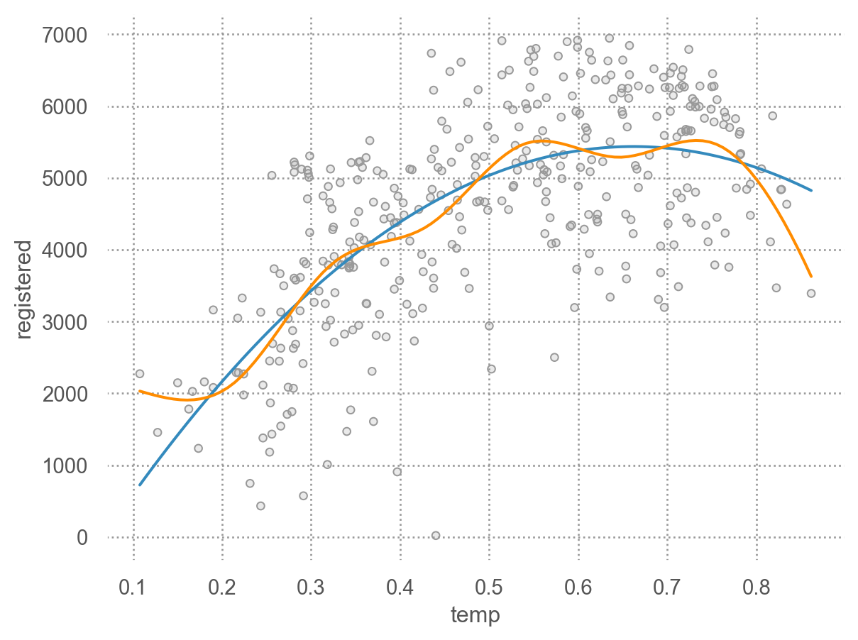
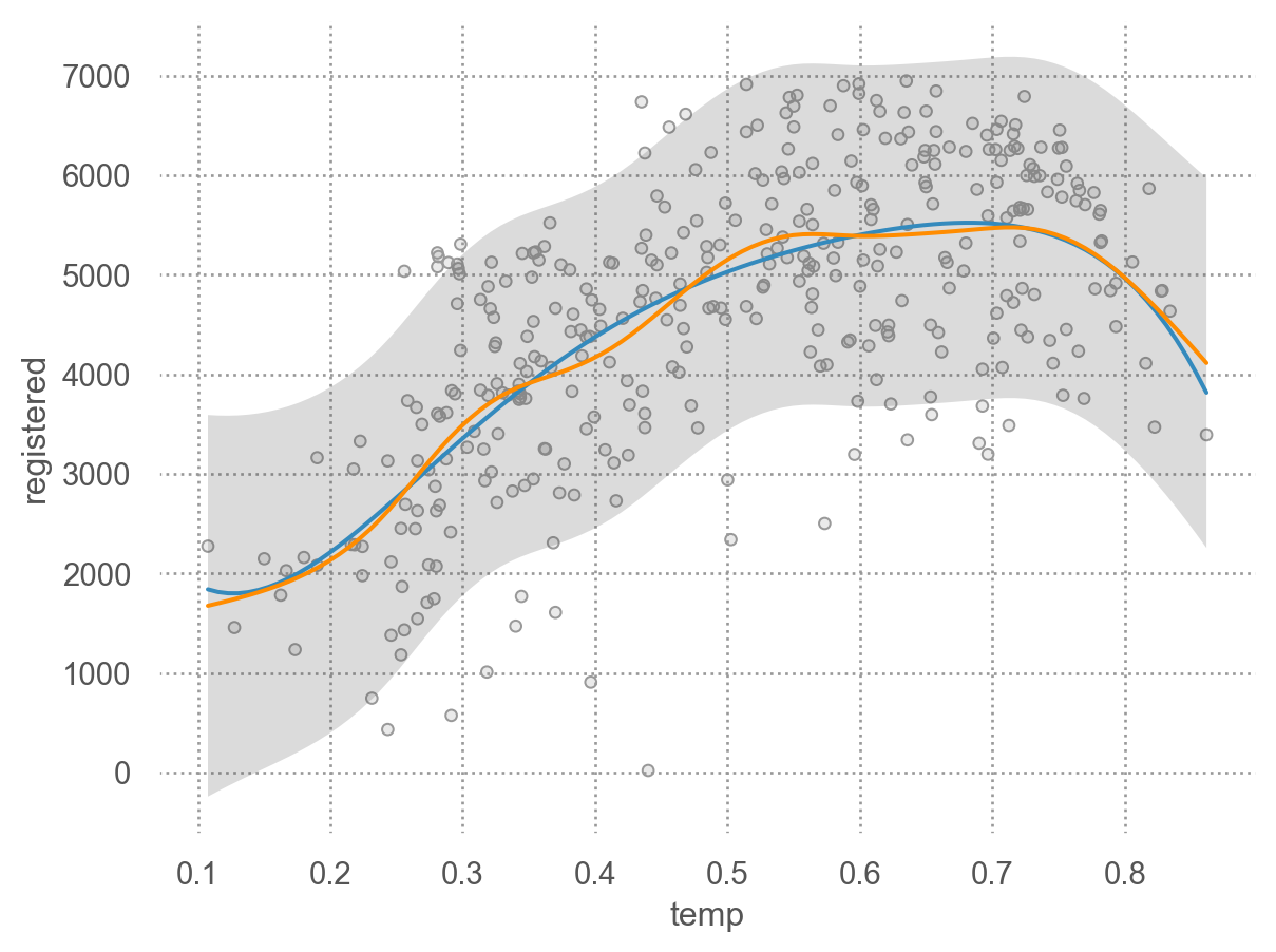
from __future__ import annotations
from dataclasses import dataclass

import numpy as np
import pandas as pd

from seaborn._stats.base import Stat

from sklearn.preprocessing import SplineTransformer
from sklearn.linear_model import LinearRegression
from sklearn.pipeline import make_pipeline

@dataclass
class SplineFit(Stat):
    """
    Fit a spline of the given n_knots and resample data onto predicted curve.
    """
    # This is a provisional class that is useful for building out functionality.
    # It may or may not change substantially in form or dissappear as we think
    # through the organization of the stats subpackage.

    n_knots: int = 5
    gridsize: int = 100

    def _fit_predict(self, data):

        x = data["x"]
        y = data["y"]
        if x.nunique() <= self.n_knots:
            # TODO warn?
            xx = yy = []
        else:
            B_basis = SplineTransformer(n_knots=self.n_knots)
            lr = LinearRegression()
            spline = make_pipeline(B_basis, lr).fit(x.values.reshape(-1, 1), y)
            xx = np.linspace(x.min(), x.max(), self.gridsize)
            yy = spline.predict(xx.reshape(-1, 1))

        return pd.DataFrame(dict(x=xx, y=yy))

    # TODO we should have a way of identifying the method that will be applied
    # and then only define __call__ on a base-class of stats with this pattern

    def __call__(self, data, groupby, orient, scales):

        return (
            groupby
            .apply(data.dropna(subset=["x", "y"]), self._fit_predict)
        )

# seaborn.objects의 객체로 변환
so.Spline = SplineFit

(
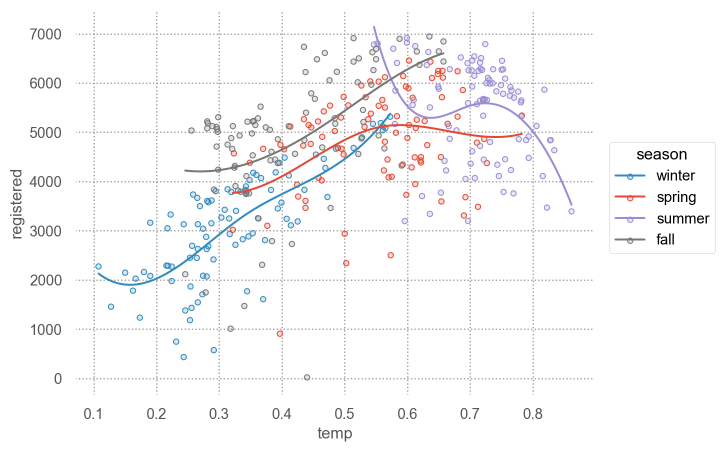
    so.Plot(bikes_daily_2012, x='temp', y='registered', color="season")
    .add(so.Dots())
    .add(so.Line(), so.Spline(3)) # Spline fit with 3 knots
)