Load packages
# numerical calculation & data frames import numpy as npimport pandas as pd# visualization import matplotlib.pyplot as pltimport seaborn as snsimport seaborn.objects as so# statistics import statsmodels.api as smimport statsmodels.formula.api as smf# pandas options 'mode.copy_on_write' , True ) # pandas 2.0 = ' {:.2f} ' .format # pd.reset_option('display.float_format') = 7 # max number of rows to display # NumPy options = 2 , suppress= True ) # suppress scientific notation # For high resolution display import matplotlib_inline"retina" )
Bike Sharing Demand
Bike Sharing in Washington D.C. Dataset
= pd.read_csv("../data/hour.csv" )= pd.read_csv("../data/day.csv" )def clean_data(df):"dteday" : "date" , "cnt" : "count" }, axis= 1 , inplace= True )= df.assign(= lambda x: pd.to_datetime(x["date" ]), # datetime type으로 변환 = lambda x: x["date" ].dt.year.astype(str ), # year 추출 = lambda x: x["date" ].dt.day_of_year, # day of the year 추출 = lambda x: x["date" ].dt.month_name().str [:3 ], # month 추출 = lambda x: x["date" ].dt.day_name().str [:3 ], # 요일 추출 "season" ] = ("season" ]map ({1 : "winter" , 2 : "spring" , 3 : "summer" , 4 : "fall" }) # season을 문자열로 변환 "category" ) # category type으로 변환 "winter" , "spring" , "summer" , "fall" ], ordered= True # 순서를 지정 return df= clean_data(bikeshare)= clean_data(bikeshare_daily)
   instant       date  season  yr  mnth  holiday  weekday  workingday  \
0        1 2011-01-01  winter   0     1        0        6           0
1        2 2011-01-02  winter   0     1        0        0           0
2        3 2011-01-03  winter   0     1        0        1           1

   weathersit  temp  atemp  hum  windspeed  casual  registered  count  year  \
0           2  0.34   0.36 0.81       0.16     331         654    985  2011
1           2  0.36   0.35 0.70       0.25     131         670    801  2011
2           1  0.20   0.19 0.44       0.25     120        1229   1349  2011

   day month wday
0    1   Jan  Sat
1    2   Jan  Sun
2    3   Jan  Mon
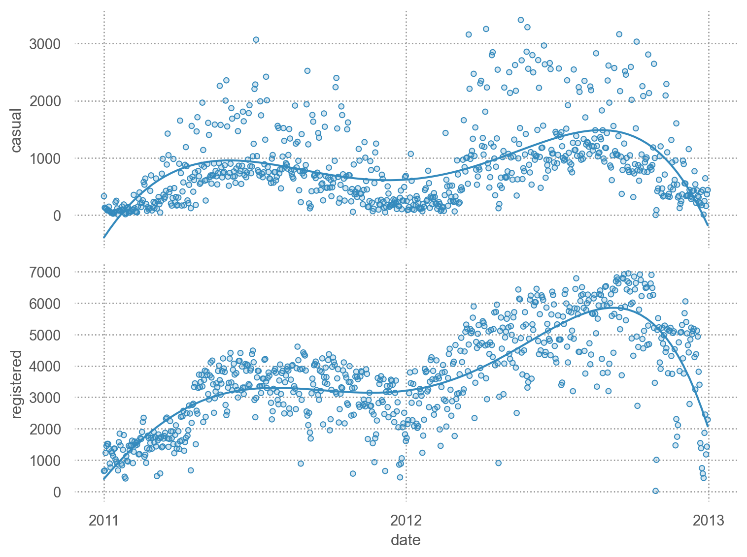
= 'date' )= ['casual' , 'registered' ])5 ))= (8 , 6 ))
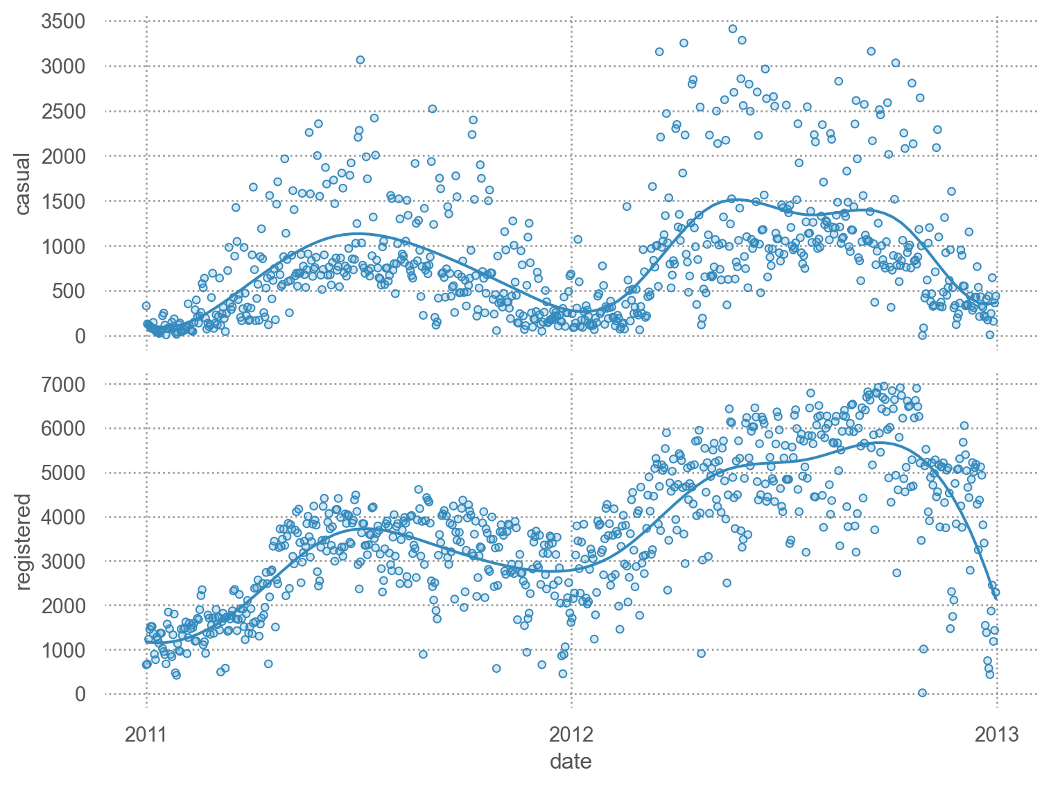
= 'date' )= ['casual' , 'registered' ])10 ))= (8 , 6 ))
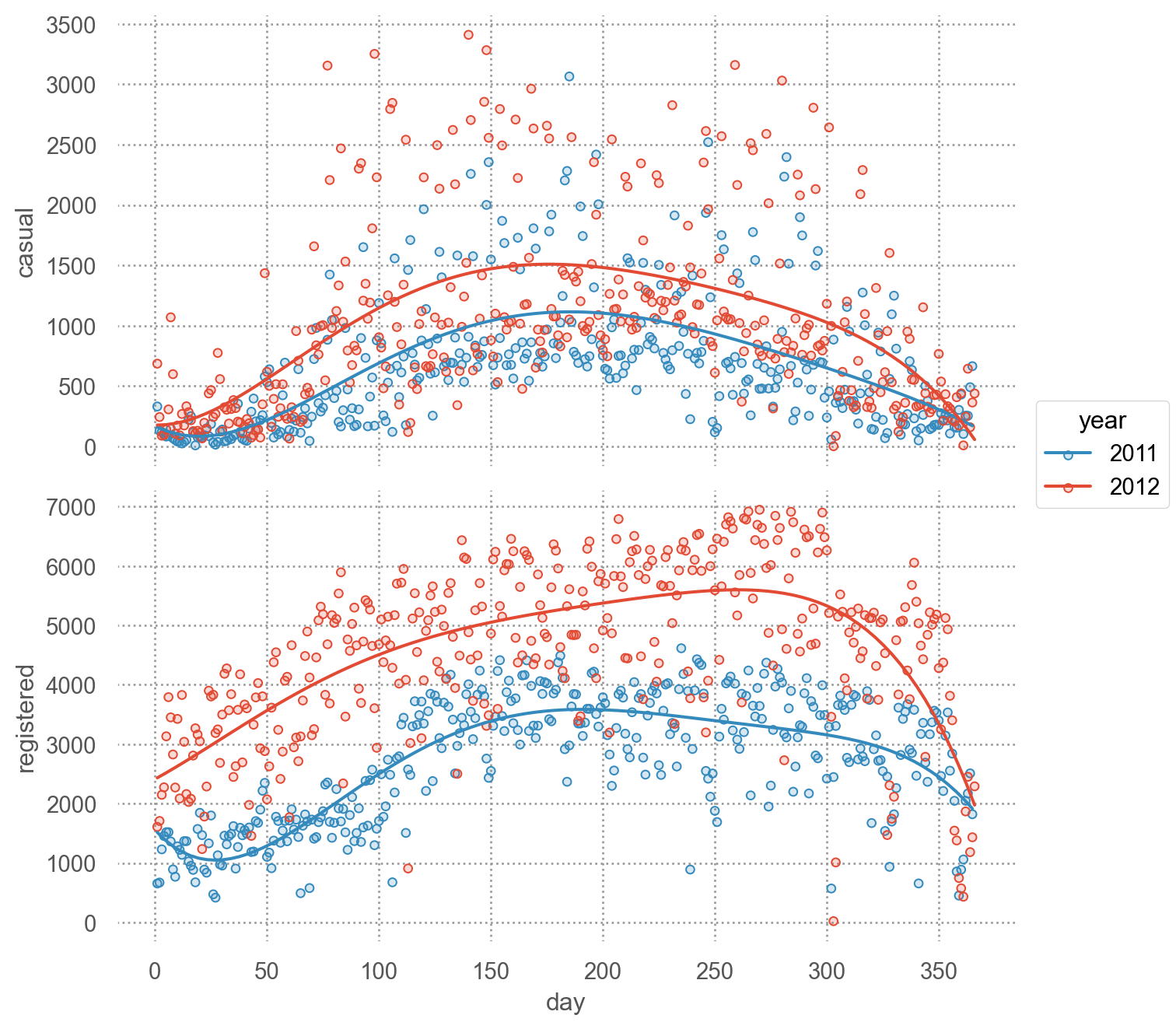
= 'day' , color= "year" )= ['casual' , 'registered' ])5 ))= (7 , 7 ))
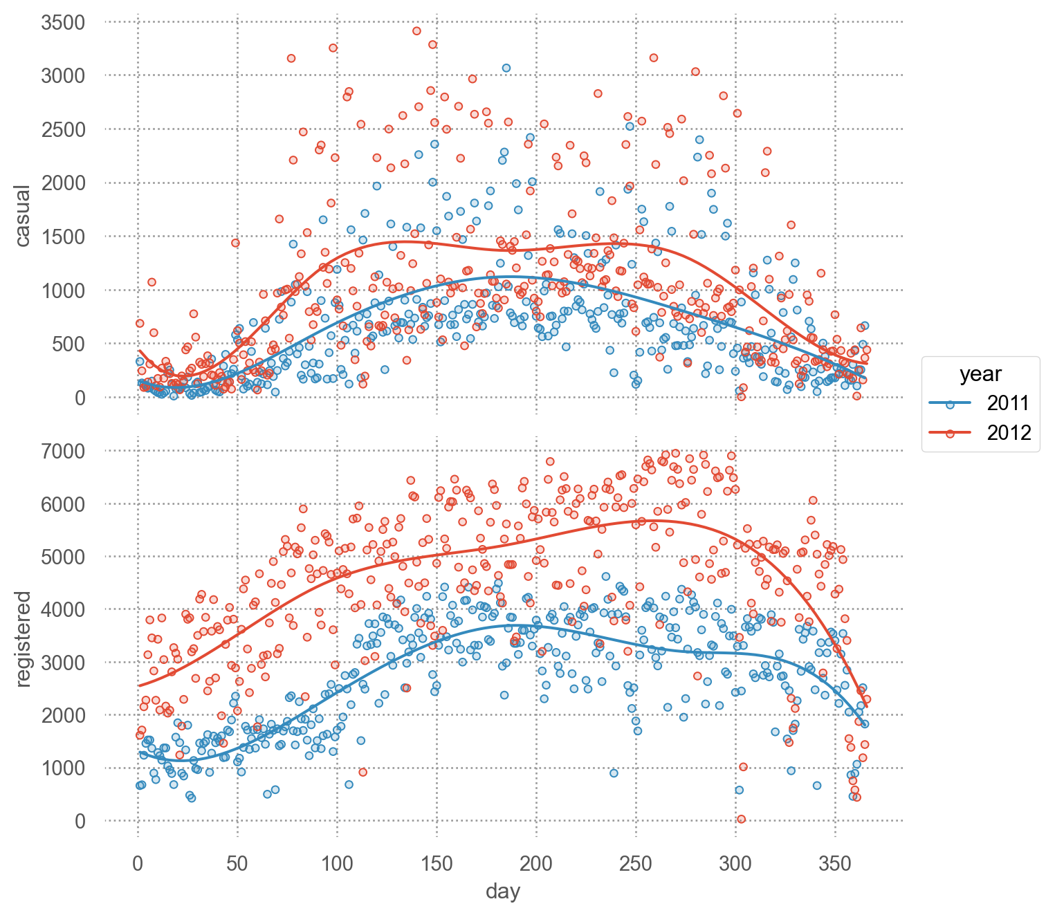
= 'day' , color= "year" )= ['casual' , 'registered' ])5 ))= (7 , 7 ))
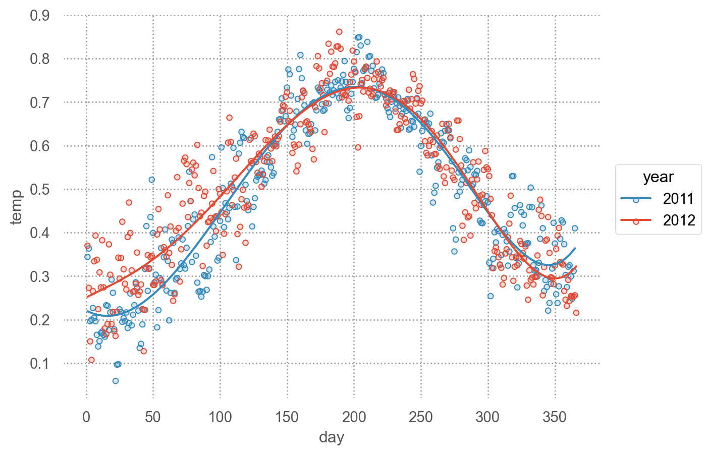
= 'day' , y= 'temp' , color= "year" )5 ))
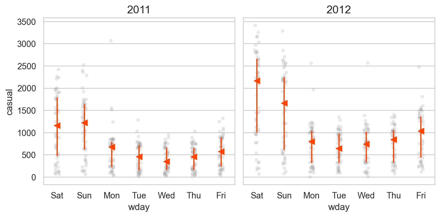
# 요일에 따라 차이가 있는가? from sbcustom import boxplot= "wday" , y= "casual" )"year" )= (8 , 4 ))
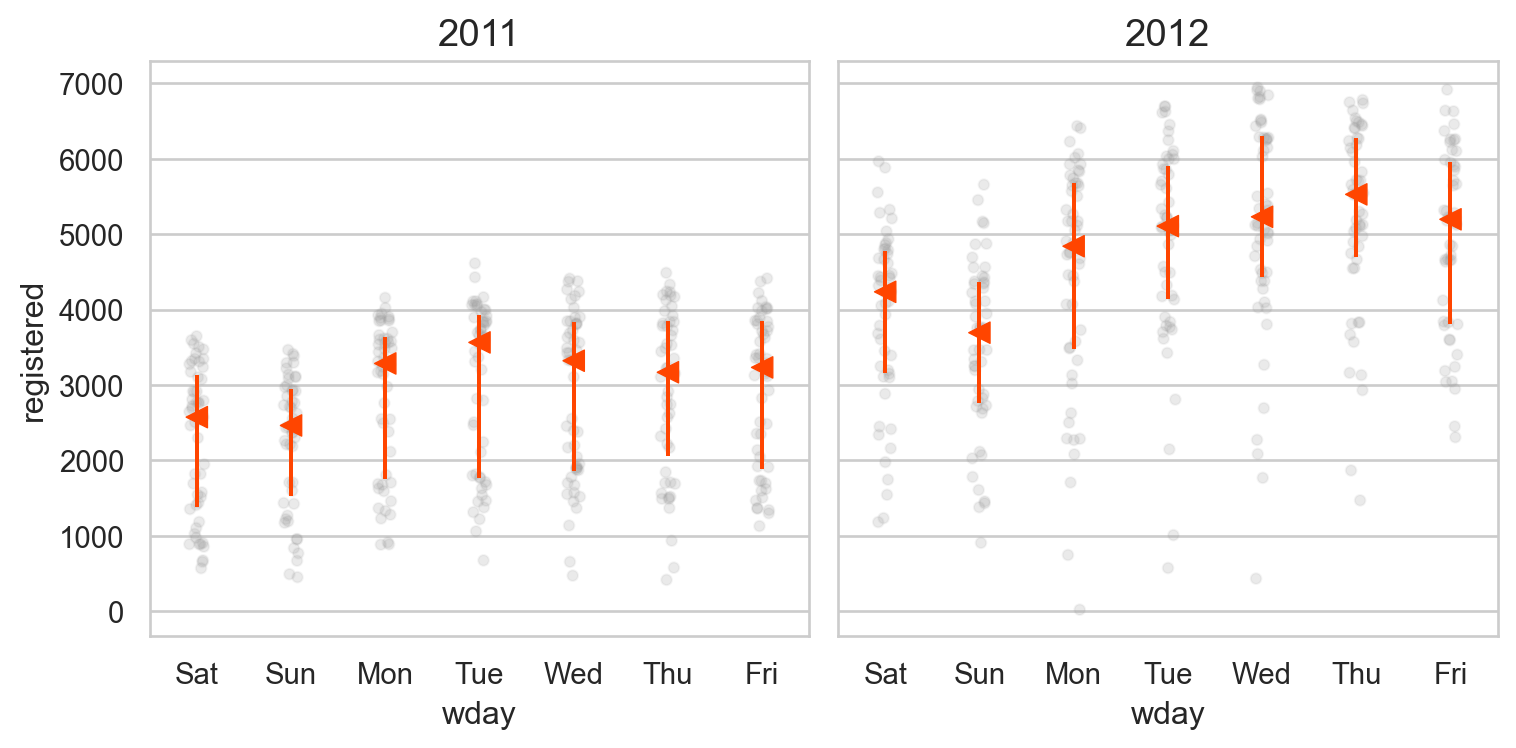
= "wday" , y= "registered" )"year" )= (8 , 4 ))
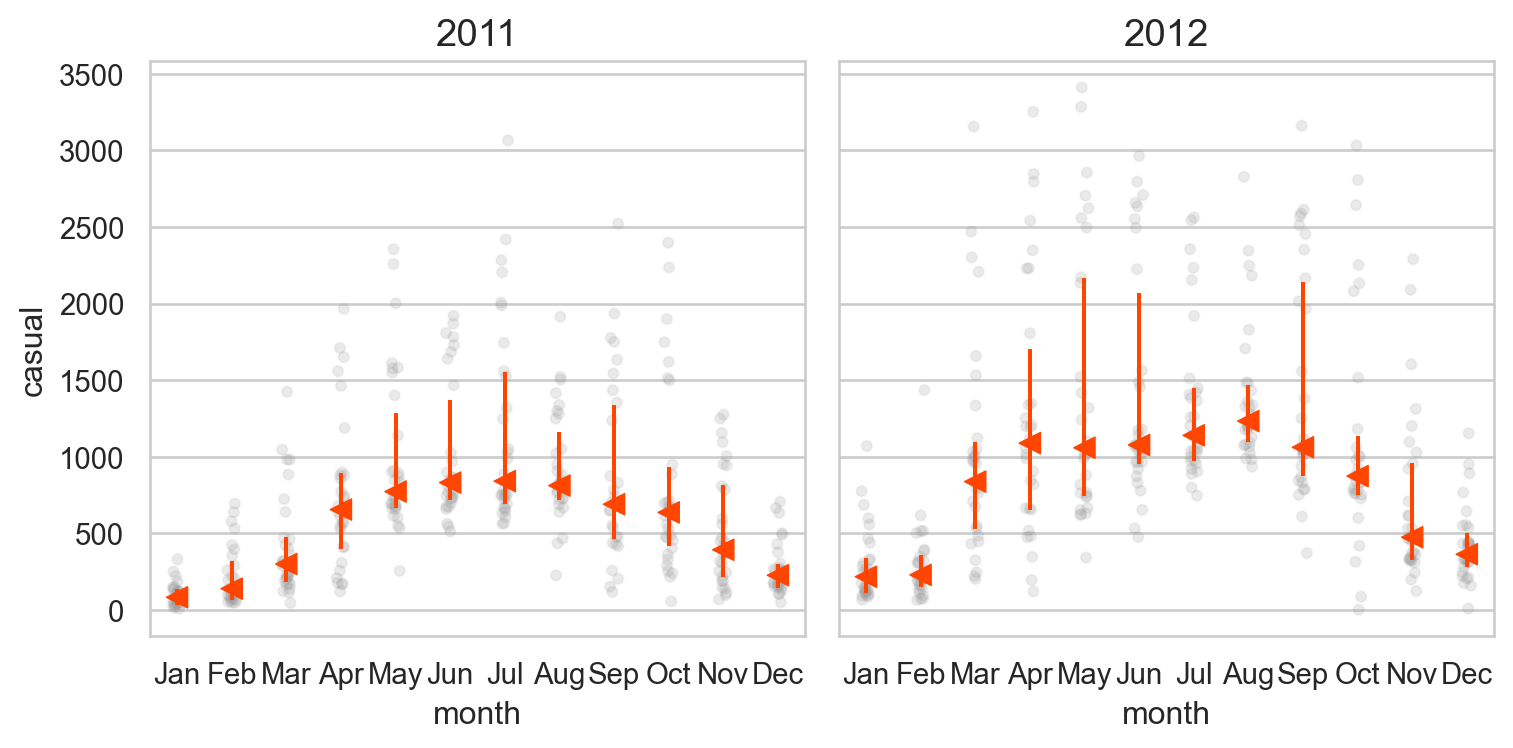
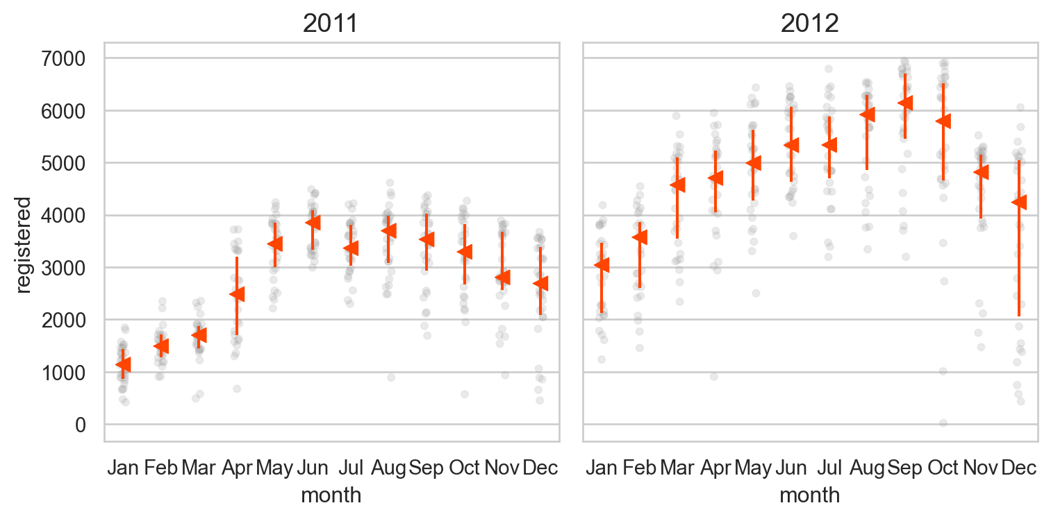
# 달에 따라 차이가 있는가? = "month" , y= "casual" )"year" )= (8 , 4 ))
= "month" , y= "registered" )"year" )= (8 , 4 ))
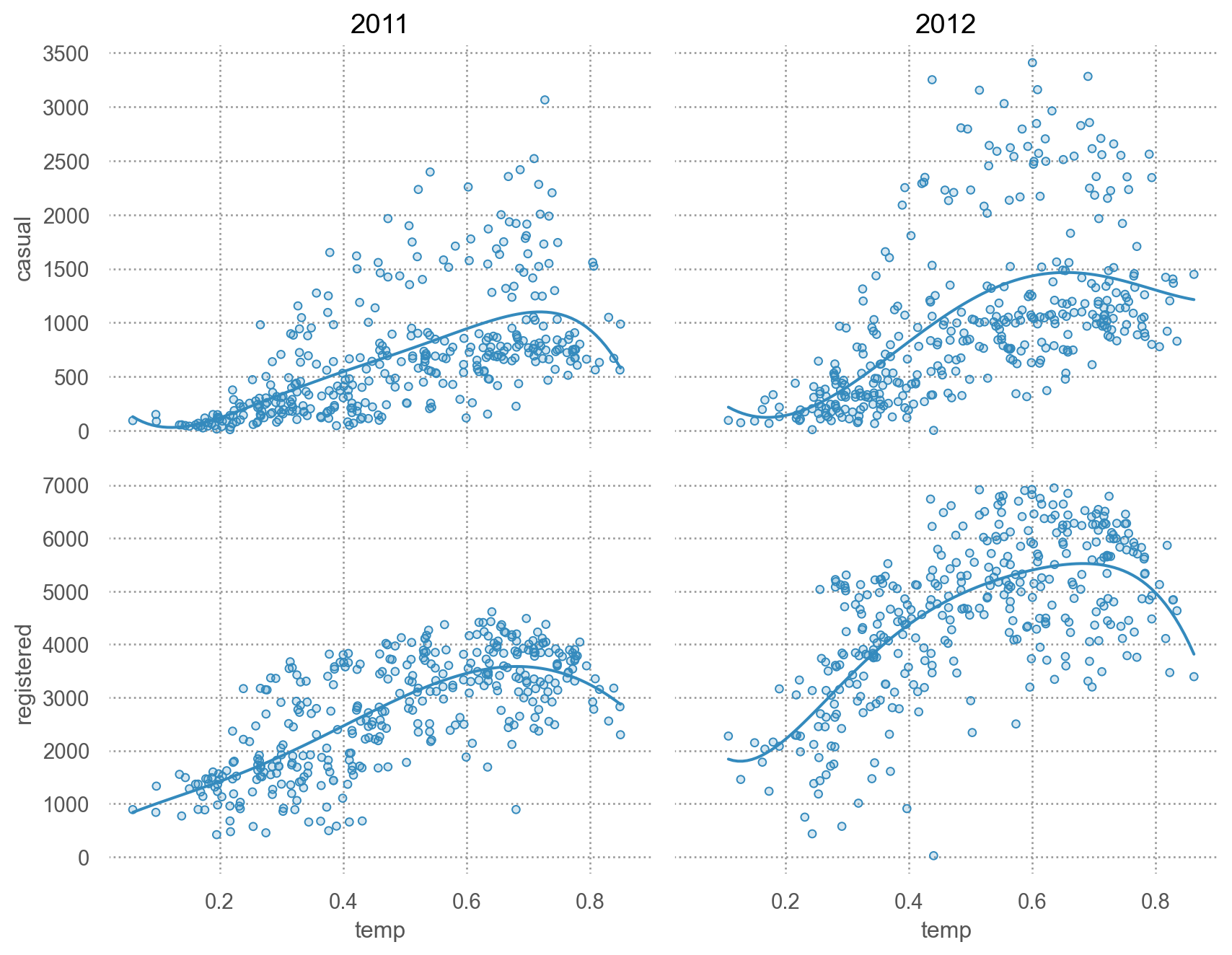
# 기온에 따라 차이가 있는가? = 'temp' )= ['casual' , 'registered' ])5 ))"year" )= (9 , 7 ))
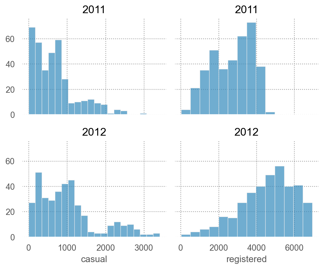
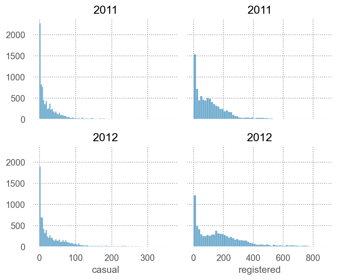
Y의 분포가 daily, hourly에 따라 매우 다름
# daily = ['casual' , 'registered' ])= "year" )= (6 , 5 ))
# hourly = ['casual' , 'registered' ])= "year" )= (6 , 5 ))
= 'temp' )= ['casual' , 'registered' ])5 ))"year" )= (9 , 7 ))
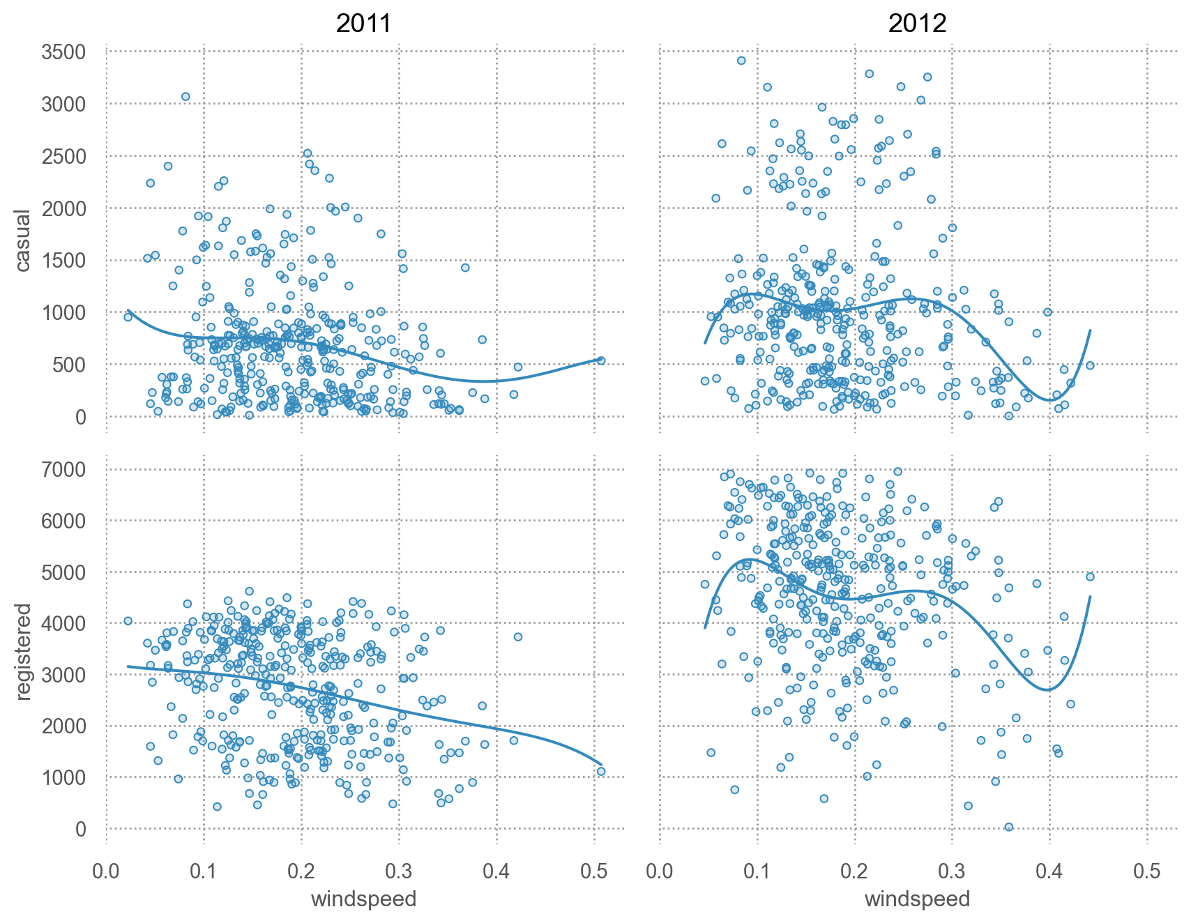
# 바람의 세기에 따라 차이가 있는가? = 'windspeed' )= ['casual' , 'registered' ])5 ))"year" )= (9 , 7 ))
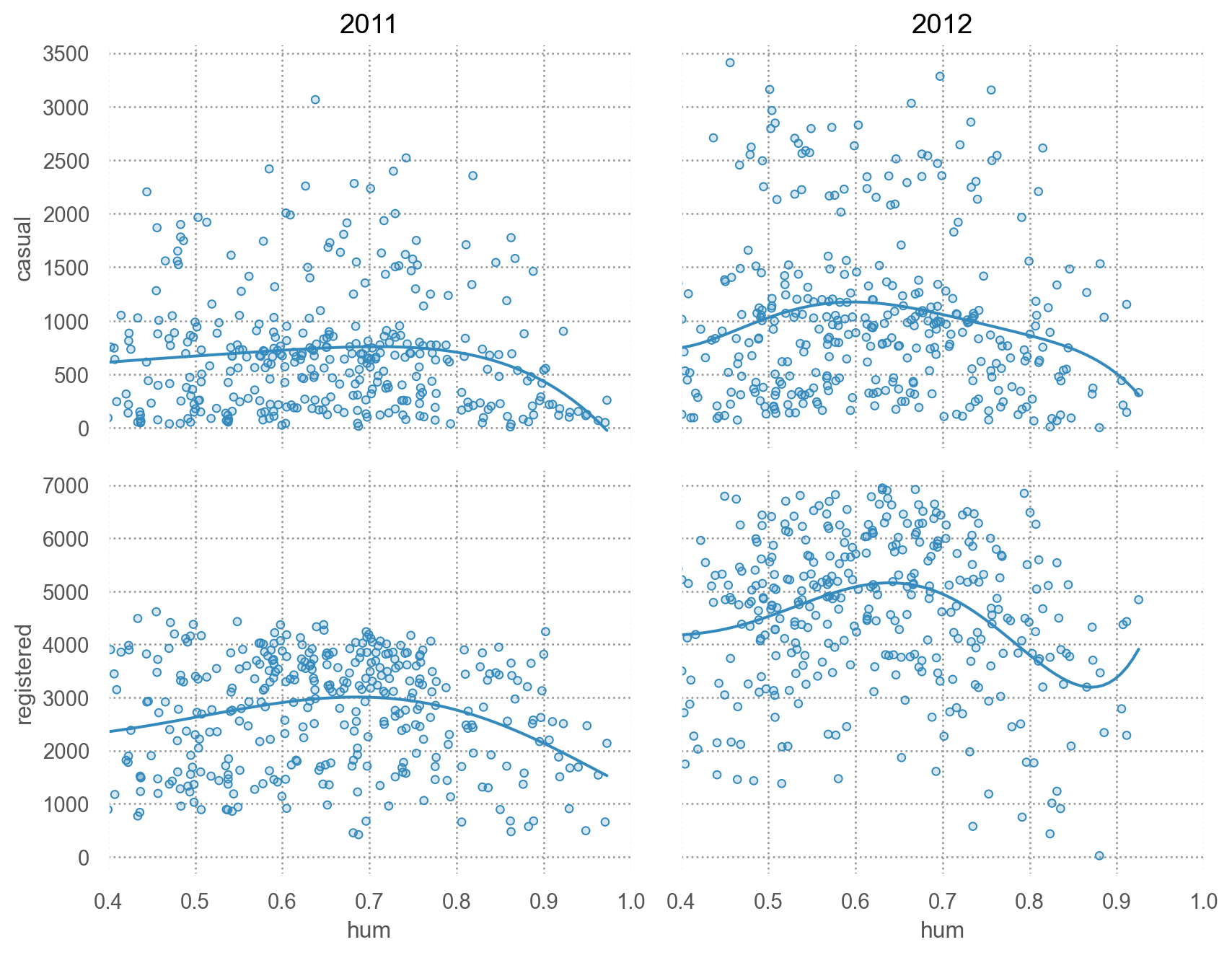
# 습도에 따라 차이가 있는가? = 'hum' )= ['casual' , 'registered' ])5 ))"year" )= (9 , 7 ))= (0.4 , 1 ))
# 기온과 습도의 관계? = 'temp' , y= 'hum' )5 ))
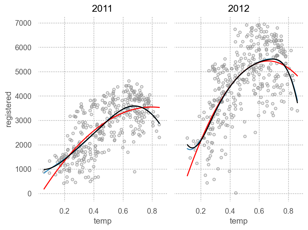
Registered bikers
= 'temp' , y= 'registered' )= ".6" ))5 ))= "red" ), so.PolyFit(2 ))= "black" ), so.Spline(5 ))"year" )
year는 예측변수로 의미는 없으나 modeling 방식의 예시를 위해 사용했음.
import statsmodels.formula.api as smf= smf.ols("registered ~ temp + I(temp**2) + year" , data= bikes_daily).fit()= smf.ols("registered ~ (temp + I(temp**2)) * year" , data= bikes_daily).fit()
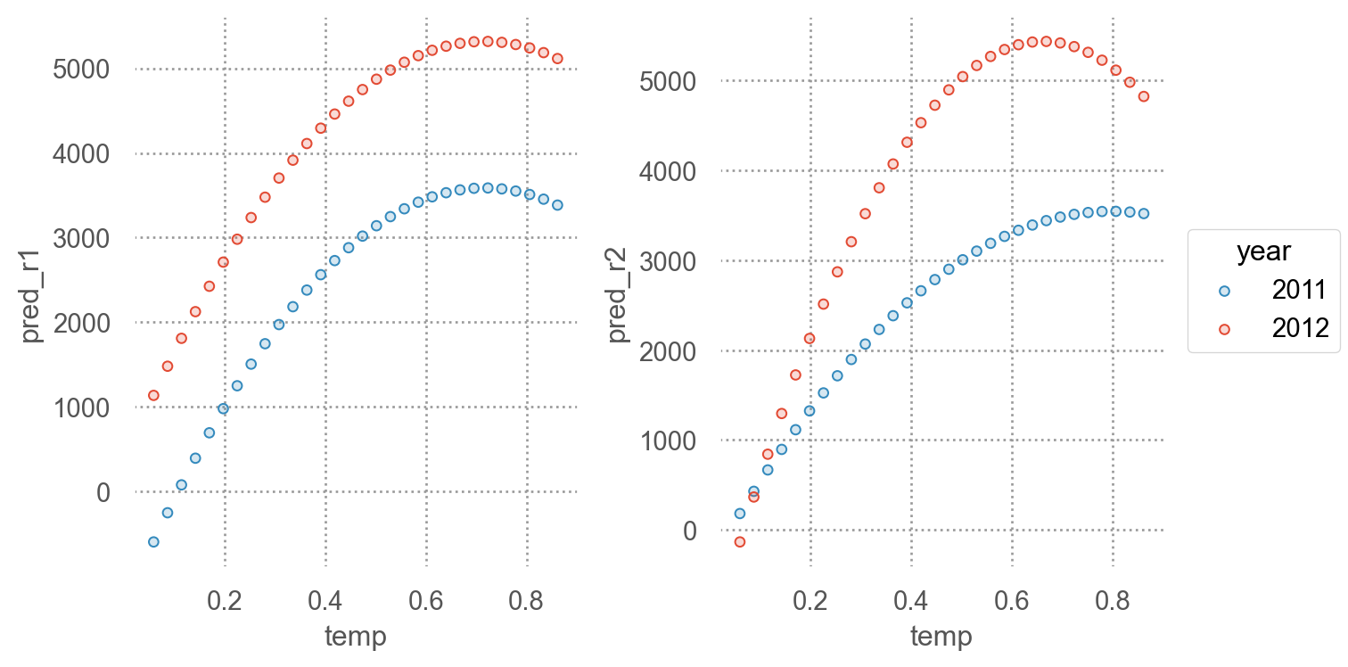
predictions
= np.linspace(bikes_daily["temp" ].min (), bikes_daily["temp" ].max (), 30 )= np.array(["2011" , "2012" ])from itertools import product= pd.DataFrame(list (product(temp, year)),= ["temp" , "year" ],"pred_r1" ] = mod_r1.predict(grid)"pred_r2" ] = mod_r2.predict(grid)= 'temp' , color= "year" )= ['pred_r1' , 'pred_r2' ], wrap= 1 )= (7 , 4 ))
residuals
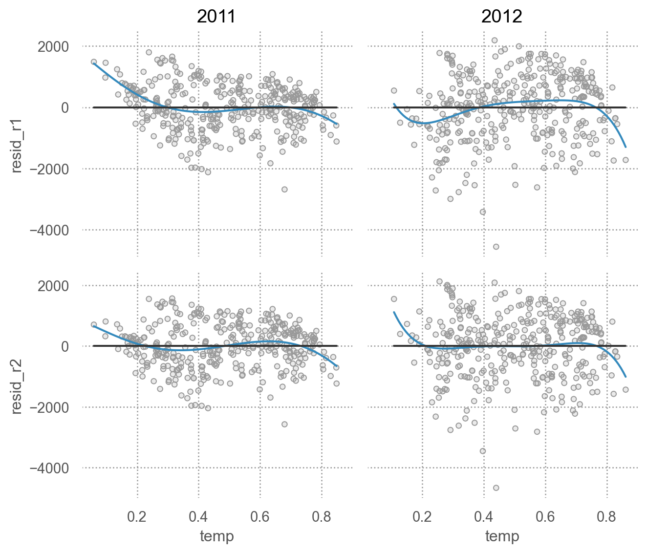
= bikes_daily.assign(= mod_r1.resid,= mod_r2.resid= 'temp' )= ['resid_r1' , 'resid_r2' ])= '.6' ))5 ))= ".2" ), so.Agg(lambda x: 0 ))"year" )= (7 , 6 ))
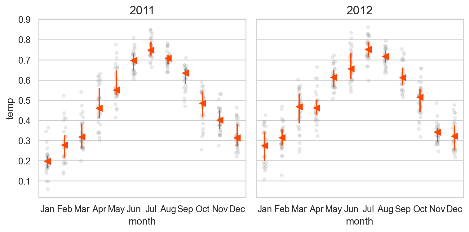
온도와 달의 밀접한 관계?
= smf.ols('temp ~ month' , data= bikes_daily).fit()
= 'month' , y= 'temp' )"year" )= (8 , 4 ))
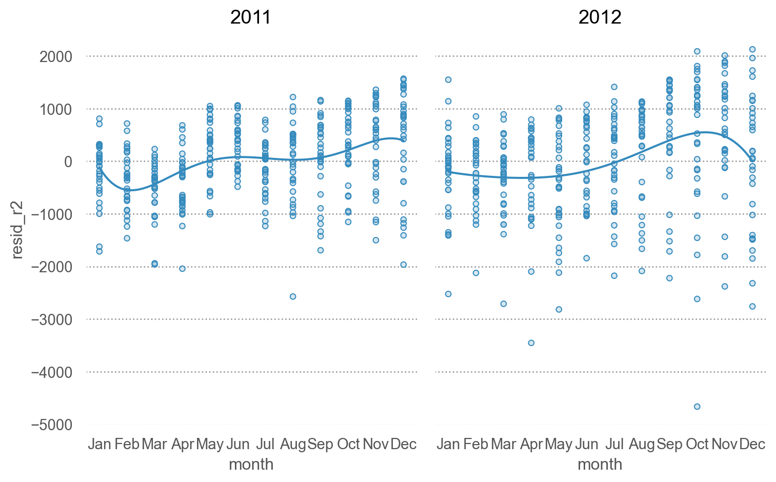
= 'month' , y= 'resid_r2' )5 ))"year" )= (8 , 5 ))
9~11월에는 온도로는 예측되지 않는, 즉 같은 온도라고 해도 자건거를 특별히 더 대여하게 되는 특성이 있을 수 있음.
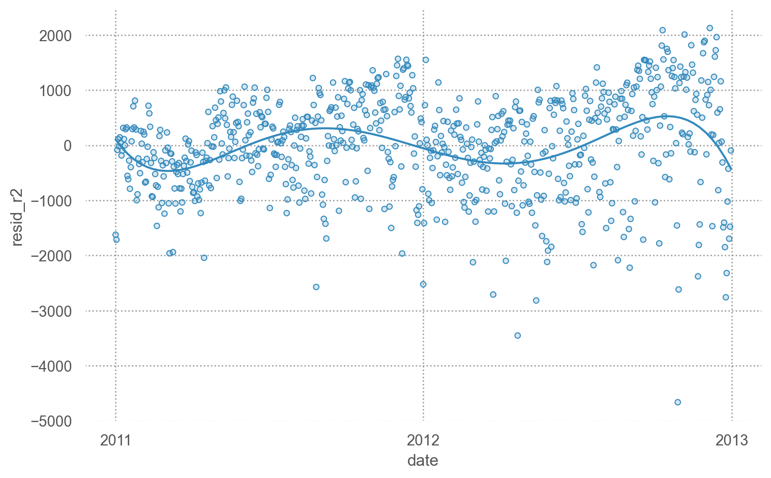
= 'date' , y= 'resid_r2' )5 )) # grouping by year = (8 , 5 ))
"month" ] = bikes_daily["month" ].astype("category" )"month" ] = bikes_daily["month" ].cat.set_categories("Jan" , "Feb" , "Mar" , "Apr" , "May" , "Jun" , "Jul" , "Aug" , "Sep" , "Oct" , "Nov" , "Dec" ]
= smf.ols("registered ~ (temp + I(temp**2)) * year + month" , data= bikes_daily).fit()
# month 추가로 인한 R2가 증가분
print (mod_r3.summary(slim= True ))
                            OLS Regression Results
==============================================================================
Dep. Variable:             registered   R-squared:                       0.705
Model:                            OLS   Adj. R-squared:                  0.699
No. Observations:                 731   F-statistic:                     106.8
Covariance Type:            nonrobust   Prob (F-statistic):          5.06e-177
=============================================================================================
                                coef    std err          t      P>|t|      [0.025      0.975]
---------------------------------------------------------------------------------------------
Intercept                   180.4223    321.376      0.561      0.575    -450.533     811.377
year[T.2012]              -1303.6849    477.877     -2.728      0.007   -2241.898    -365.472
month[T.Feb]                 16.8031    163.242      0.103      0.918    -303.688     337.295
month[T.Mar]                 70.8817    178.488      0.397      0.691    -279.542     421.306
month[T.Apr]                291.0581    198.194      1.469      0.142     -98.054     680.170
month[T.May]                649.9687    223.994      2.902      0.004     210.202    1089.735
month[T.Jun]               1021.8253    248.544      4.111      0.000     533.861    1509.789
month[T.Jul]                853.7900    277.468      3.077      0.002     309.039    1398.541
month[T.Aug]                985.2750    256.593      3.840      0.000     481.508    1489.041
month[T.Sep]               1085.0183    229.970      4.718      0.000     633.521    1536.516
month[T.Oct]                995.3377    200.849      4.956      0.000     601.012    1389.663
month[T.Nov]                946.3073    178.028      5.315      0.000     596.786    1295.828
month[T.Dec]                568.6507    166.184      3.422      0.001     242.382     894.919
temp                       6120.3556   1655.969      3.696      0.000    2869.205    9371.506
temp:year[T.2012]           1.24e+04   2087.372      5.938      0.000    8297.289    1.65e+04
I(temp ** 2)              -3876.2985   1731.986     -2.238      0.026   -7276.693    -475.904
I(temp ** 2):year[T.2012] -1.105e+04   2082.530     -5.304      0.000   -1.51e+04   -6958.058
=============================================================================================

Notes:
[1] Standard Errors assume that the covariance matrix of the errors is correctly specified.
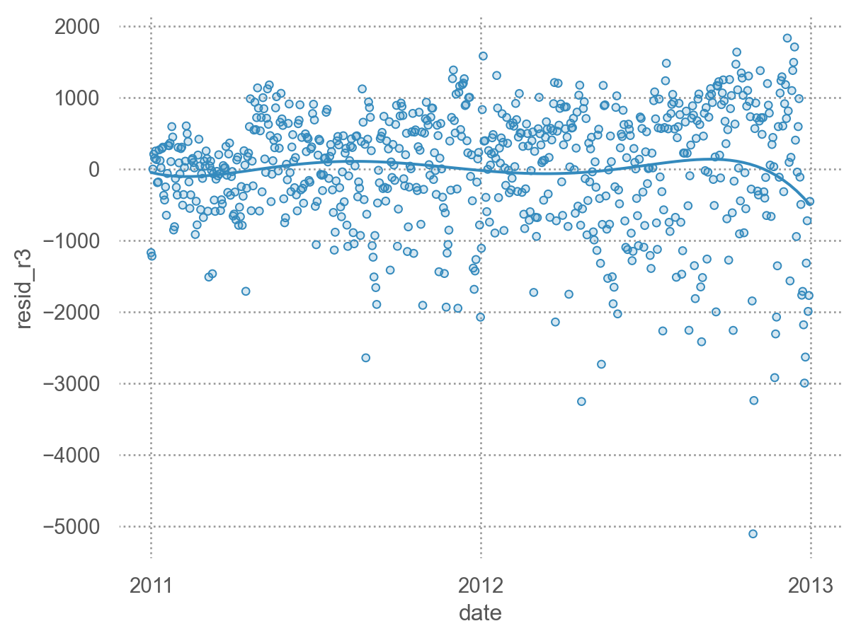
"resid_r3" ] = mod_r3.resid
= 'date' , y= 'resid_r3' )5 ))
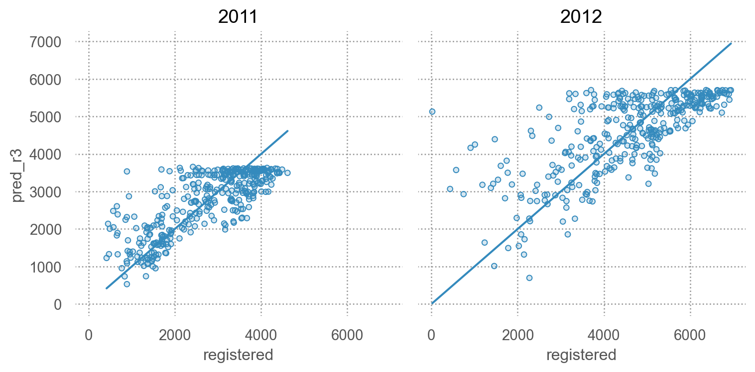
# 예측값과 실제값 비교 "pred_r3" ] = mod_r3.predict(bikes_daily)= 'registered' , y= 'pred_r3' )= 'registered' )"year" )= (8 , 4 ))
= bikes_daily_resid.query('resid_r3 < -2000' )[["date" , "holiday" ]]
          date  holiday
238 2011-08-27        0
365 2012-01-01        0
448 2012-03-24        0
477 2012-04-22        0
499 2012-05-14        0
517 2012-06-01        0
567 2012-07-21        0
596 2012-08-19        0
610 2012-09-02        0
626 2012-09-18        0
645 2012-10-07        0
667 2012-10-29        0
668 2012-10-30        0
691 2012-11-22        1
692 2012-11-23        0
693 2012-11-24        0
723 2012-12-24        0
724 2012-12-25        1
725 2012-12-26        0
모형의 비교와 각 예측변수의 공헌도
= smf.ols("registered ~ year" , data= bikes_daily).fit()= smf.ols("registered ~ year + temp + I(temp**2)" , data= bikes_daily).fit()= smf.ols("registered ~ year + temp + I(temp**2) + month" , data= bikes_daily).fit()= smf.ols("registered ~ year + temp + I(temp**2) + month + wday" , data= bikes_daily).fit()print (f" year: { mod_r_year. rsquared:.3f} \n " ,f"year + temperature: { mod_r_temp. rsquared:.3f} \n " ,f"year + temperature + months: { mod_r_month. rsquared:.3f} \n " ,f"year + temperature + months + days of the week: { mod_r_wday. rsquared:.3f} " ,
 year: 0.353
 year + temperature: 0.653
 year + temperature + months: 0.686
 year + temperature + months + days of the week: 0.757
Casual bikers
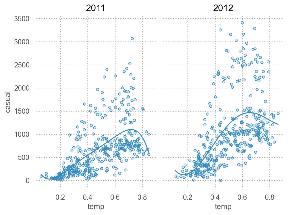
= 'temp' , y= 'casual' )5 ))"year" )
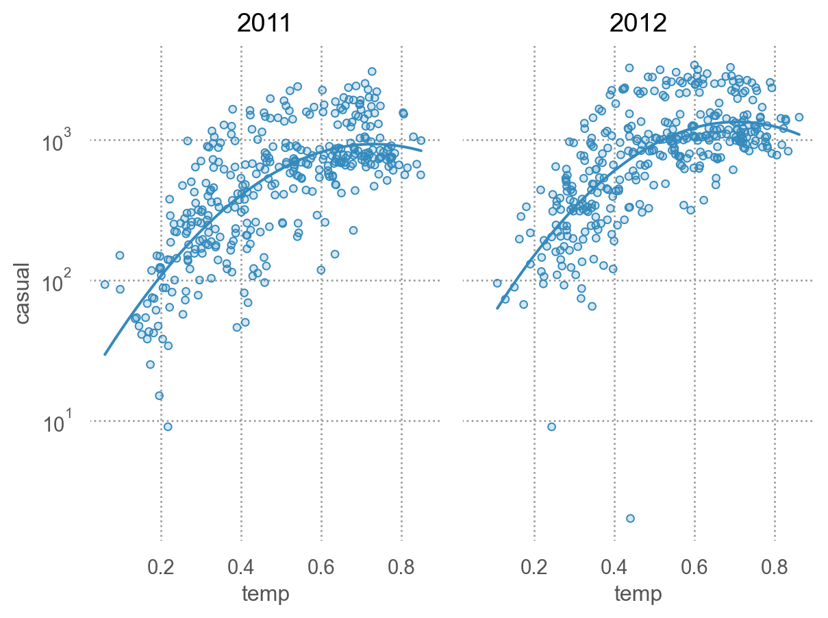
# log scale for y = 'temp' , y= 'casual' )2 ))"year" )= "log" ) # log scale
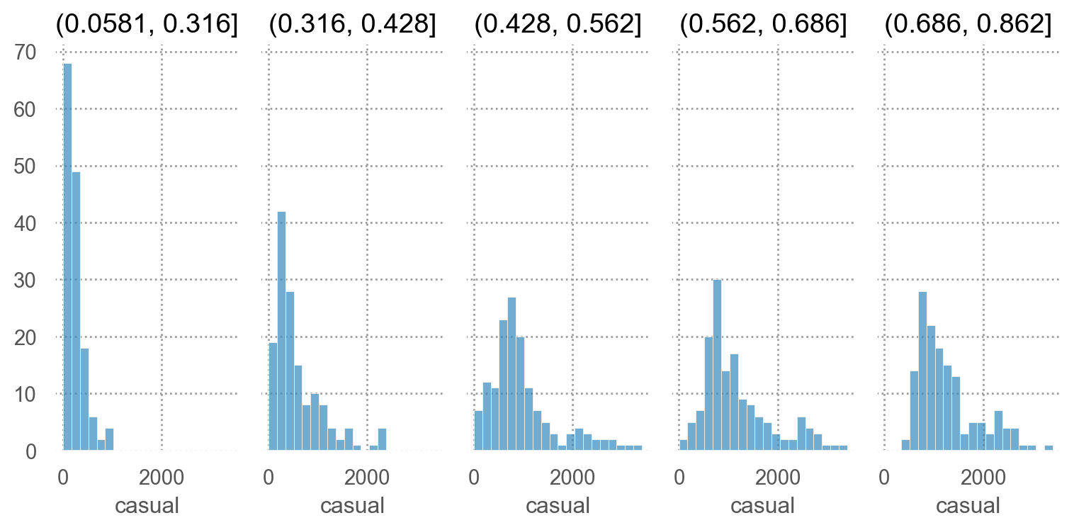
# 온도를 5개 구간으로 나누어 각 온도구간에서의 분포를 살펴봄 "temp_cat" ] = pd.qcut(bikes_daily["temp" ], 5 )= 'casual' )"temp_cat" )= (8 , 4 ))
"temp_cat" ] = pd.qcut(bikes_daily["temp" ], 7 )= lambda x: x.casual / 100 ).groupby("temp_cat" )["casual2" ].agg(["mean" , "var" ])
                 mean   var
temp_cat
(0.0581, 0.281]  1.94  2.54
(0.281, 0.355]   4.33  9.42
(0.355, 0.447]   6.74 38.09
(0.447, 0.544]  10.11 46.18
(0.544, 0.635]  11.71 58.61
(0.635, 0.716]  12.67 42.25
(0.716, 0.862]  11.88 29.46
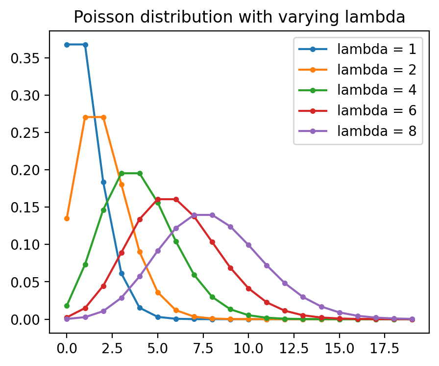
이렇게 count 데이터가 전형적으로 보이는 “평균에 따라 표준편차가 함께 증가”하는 경우, generalized linear model (GLM)의 하나인 포아송(Poisson) 분포나 이를 보정한 다른 분포를 결합한 모형을 이용하는 것이 권장됨.
Y를 transform하는 것보다 여러 이점이 있는 한편, Y가 내재적으로 log나 sqrt의 의미를 띤다면 transform하는 것이 더 적절할 수도 있음.
"lcasual" ] = np.log2(bikes_daily["casual" ] + 1 )
= smf.ols("lcasual ~ (temp + I(temp**2)) + year" , data= bikes_daily).fit()
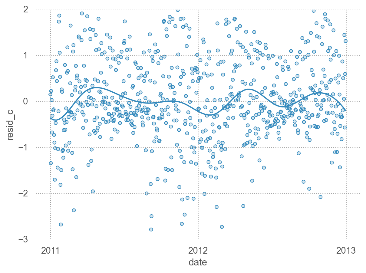
"resid_c" ] = mod_c.resid"lcasual" ] = np.log2(bikes_daily_resid["casual" ] + 1 )
= 'date' , y= 'resid_c' )10 ))= (- 3 , 2 ))
# 요일에 따라 차이가 있는가? from sbcustom import boxplot= "wday" , y= "casual" )"year" )= (8 , 4 ))
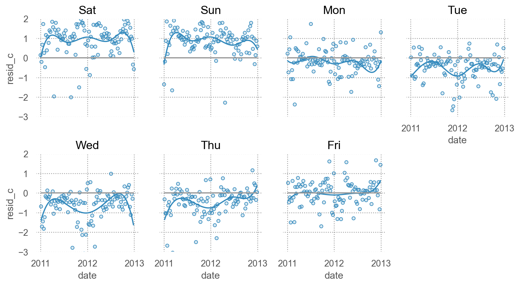
요일의 차이가 추가적으로 설명할 수 있는 부분이 있는가?
= 'date' , y= 'resid_c' )5 ))= ".6" ), so.Agg(lambda x: 0 ))= (- 3 , 2 ))"wday" , wrap= 4 )= (9 , 5 ))
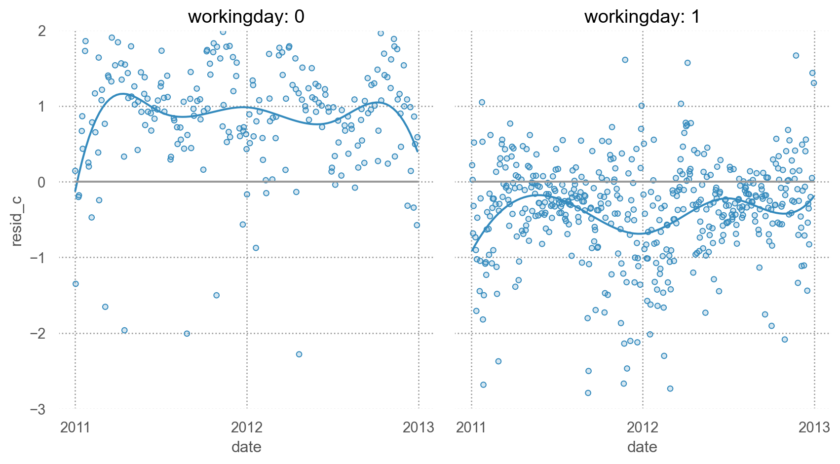
= 'date' , y= 'resid_c' )5 ))= ".6" ), so.Agg(lambda x: 0 ))= (- 3 , 2 ))"workingday" )= (9 , 5 ))= "workingday: {} " .format )
요일별로 모두 고려할 것인가? 아니면 평일/주말로 나눌 것인가?
# 요일별로 = smf.ols("lcasual ~ (temp + I(temp**2)) + year + wday" , data= bikes_daily).fit()# 평일/주말 = smf.ols("lcasual ~ (temp + I(temp**2)) + year + workingday" , data= bikes_daily).fit()# 습도 추가 = smf.ols("lcasual ~ (temp + I(temp**2)) + year + wday + bs(hum, 4)" , data= bikes_daily).fit()
= sm.RLM.from_formula("lcasual ~ (temp + I(temp**2)) + year + wday + bs(hum, 4)" , data= bikes_daily).fit()
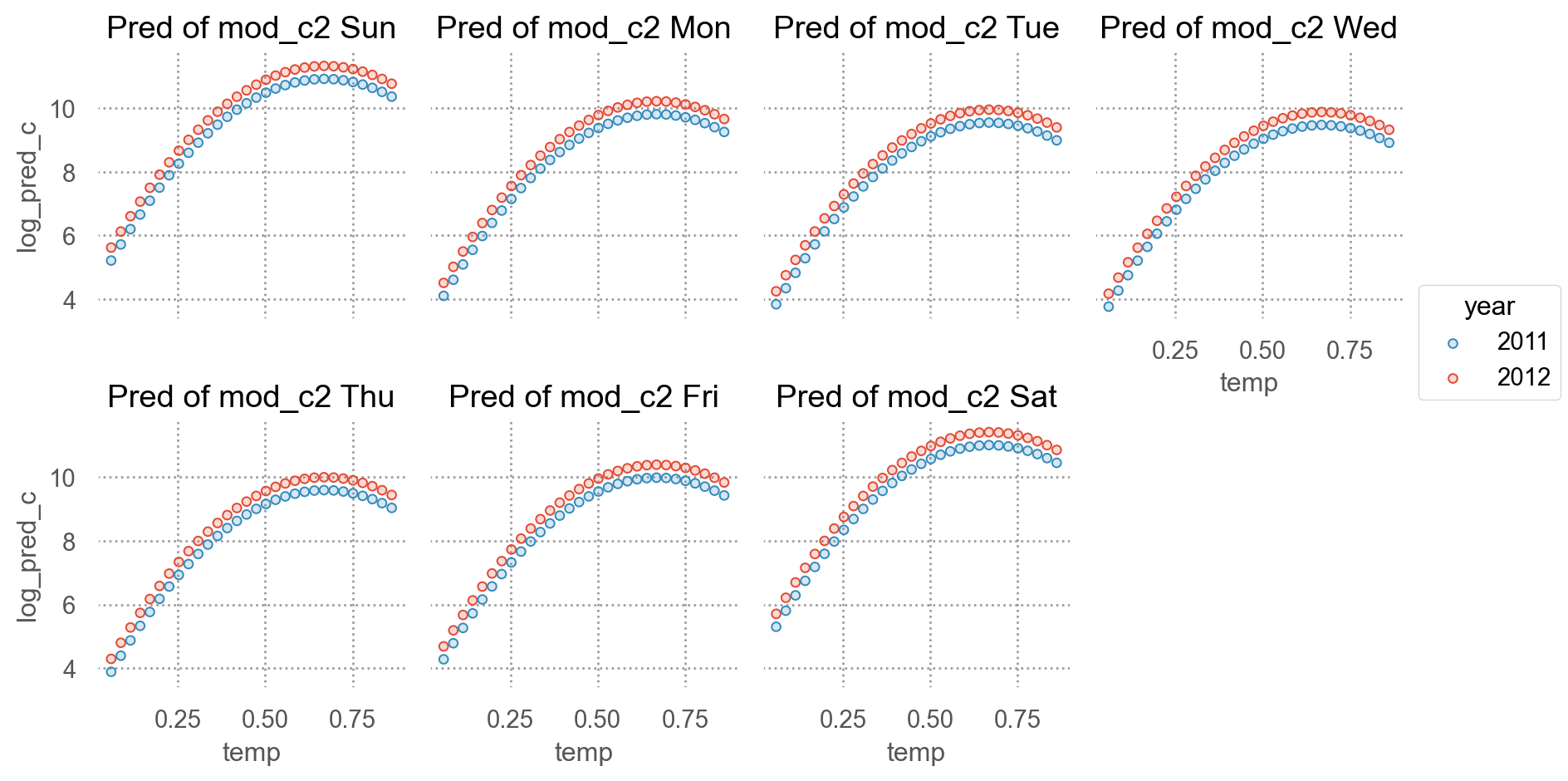
마지막 모형(mod_c2)의 예측값smf.ols("lcasual ~ (temp + I(temp**2)) + year + wday + bs(hum, 4)", data=bikes_daily)
predictions
= np.linspace(bikes_daily["temp" ].min (), bikes_daily["temp" ].max (), 30 )= np.array([bikes_daily["hum" ].mean()])= np.array(["2011" , "2012" ])= np.array(["Sun" , "Mon" , "Tue" , "Wed" , "Thu" , "Fri" , "Sat" ])from itertools import product= pd.DataFrame(list (product(temp, year, wday, hum)),= ["temp" , "year" , "wday" , "hum" ],"log_pred_c" ] = mod_c3.predict(grid)= 'temp' , y= 'log_pred_c' , color= "year" )"wday" , wrap= 4 )= "Pred of mod_c2 {} " .format )= (9 , 5 ))
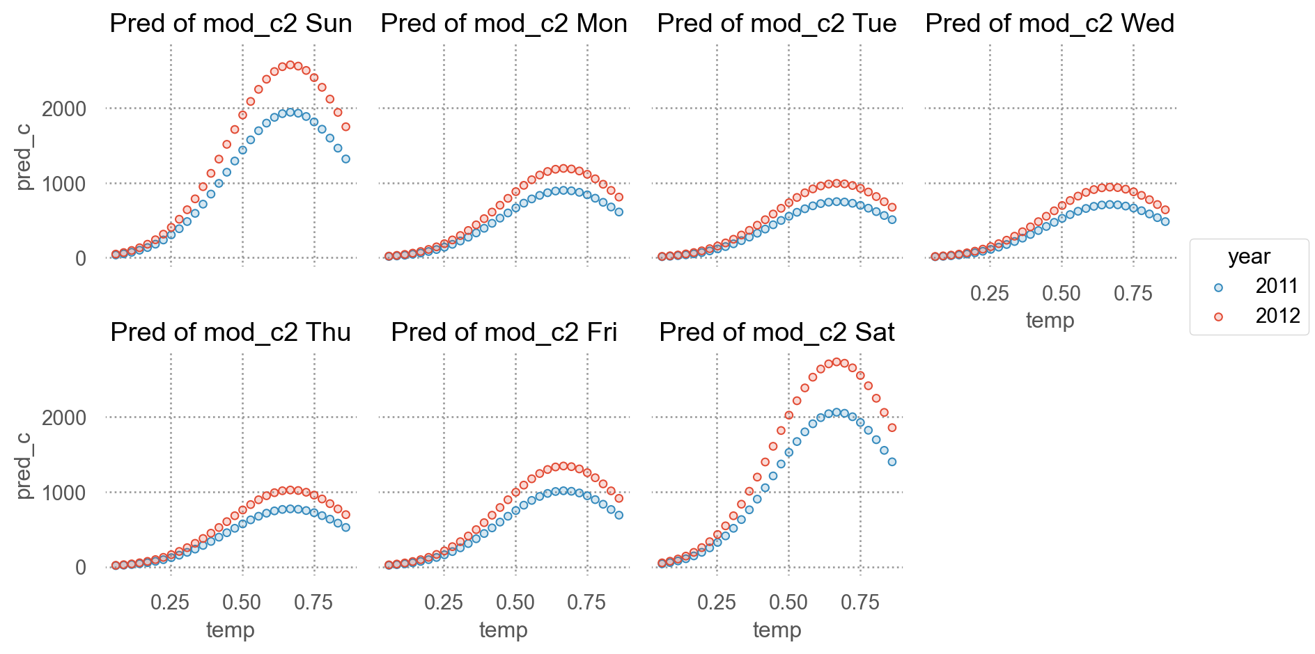
Original scale로 예측값
predictions with the original scale
= np.linspace(bikes_daily["temp" ].min (), bikes_daily["temp" ].max (), 30 )= np.array([bikes_daily["hum" ].mean()])= np.array(["2011" , "2012" ])= np.array(["Sun" , "Mon" , "Tue" , "Wed" , "Thu" , "Fri" , "Sat" ])from itertools import product= pd.DataFrame(list (product(temp, year, wday, hum)),= ["temp" , "year" , "wday" , "hum" ],"pred_c" ] = 2 ** mod_c3.predict(grid) - 1 = 'temp' , y= 'pred_c' , color= "year" )"wday" , wrap= 4 )= "Pred of mod_c2 {} " .format )= (9 , 5 ))
잔차 확인
"resid_c2" ] = mod_c2.resid"resid_c3" ] = mod_c3.resid
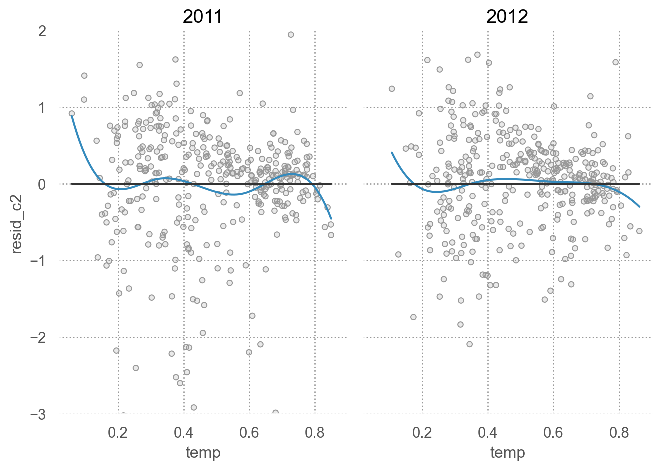
residual plot for mod_c2; 습도 추가 전
= 'temp' , y= 'resid_c2' )= '.6' ))4 ))= ".2" ), so.Agg(lambda x: 0 ))"year" )= (7 , 5 ))= (- 3 , 2 ))
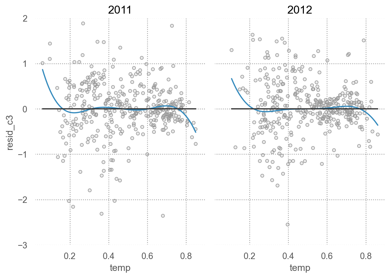
residual plot for mod_c3; 습도까지 포함
= 'temp' , y= 'resid_c3' )= '.6' ))4 ))= ".2" ), so.Agg(lambda x: 0 ))"year" )= (7 , 5 ))= (- 3 , 2 ))
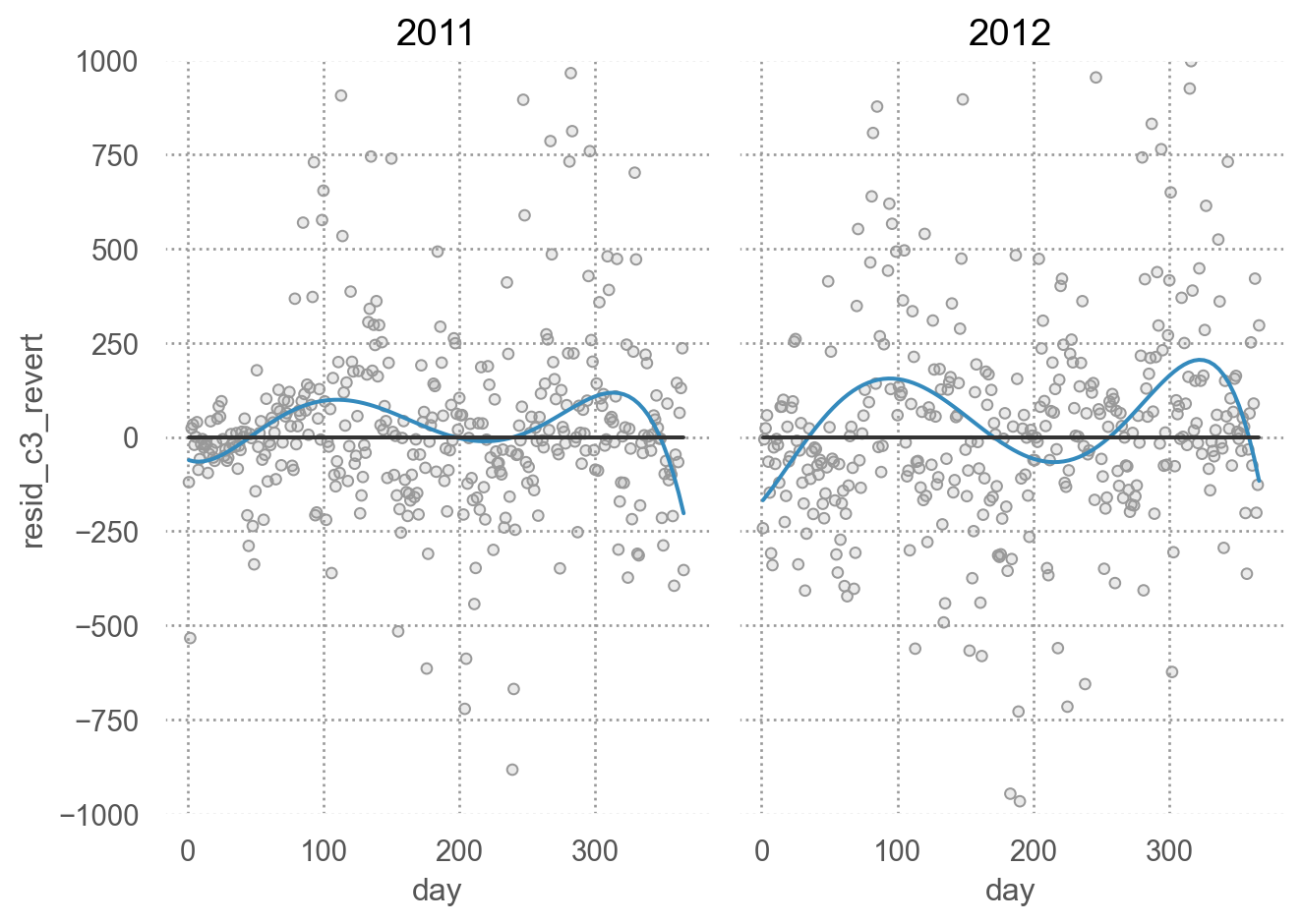
residual with the original scale
= bikes_daily.assign(= lambda x: 2 ** mod_c3.predict(x) - 1 ,= lambda x: x["casual" ] - x["pred_c3_revert" ]= 'day' , y= 'resid_c3_revert' )= '.6' ))5 ))= ".2" ), so.Agg(lambda x: 0 ))"year" )= (7 , 5 ))= (- 1000 , 1000 ))
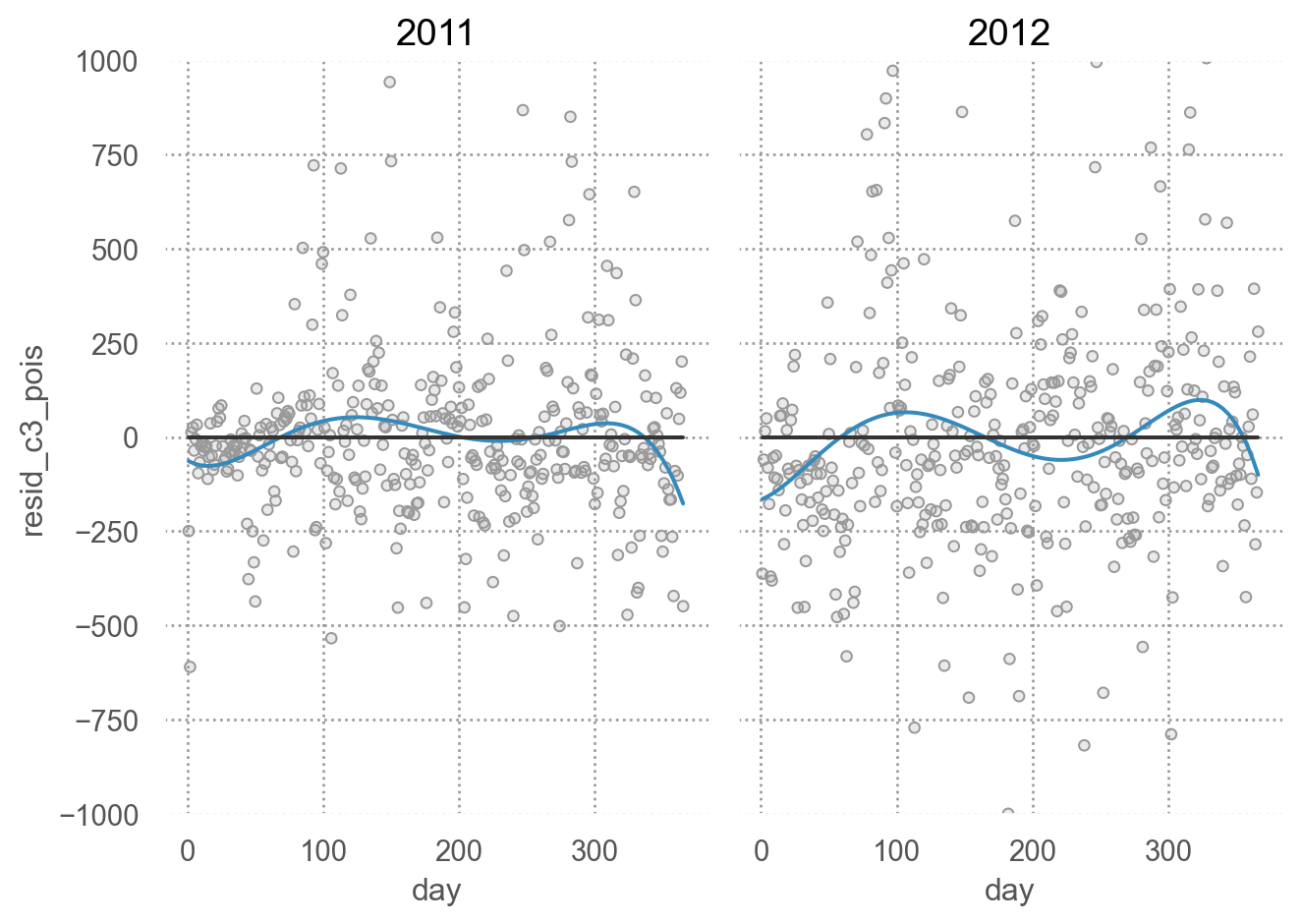
Poissong regresion residuals
# poisson regression = smf.poisson("casual ~ (temp + I(temp**2)) + year + wday + bs(hum, 5)" , data= bikes_daily).fit()"resid_c3_pois" ] = mod_c3_pois.resid"pred_c3_pois" ] = mod_c3_pois.predict(bikes_daily)= 'day' , y= 'resid_c3_pois' )= '.6' ))5 ))= ".2" ), so.Agg(lambda x: 0 ))"year" )= (7 , 5 ))= (- 1000 , 1000 ))
Optimization terminated successfully.
         Current function value: 49.152525
         Iterations 7
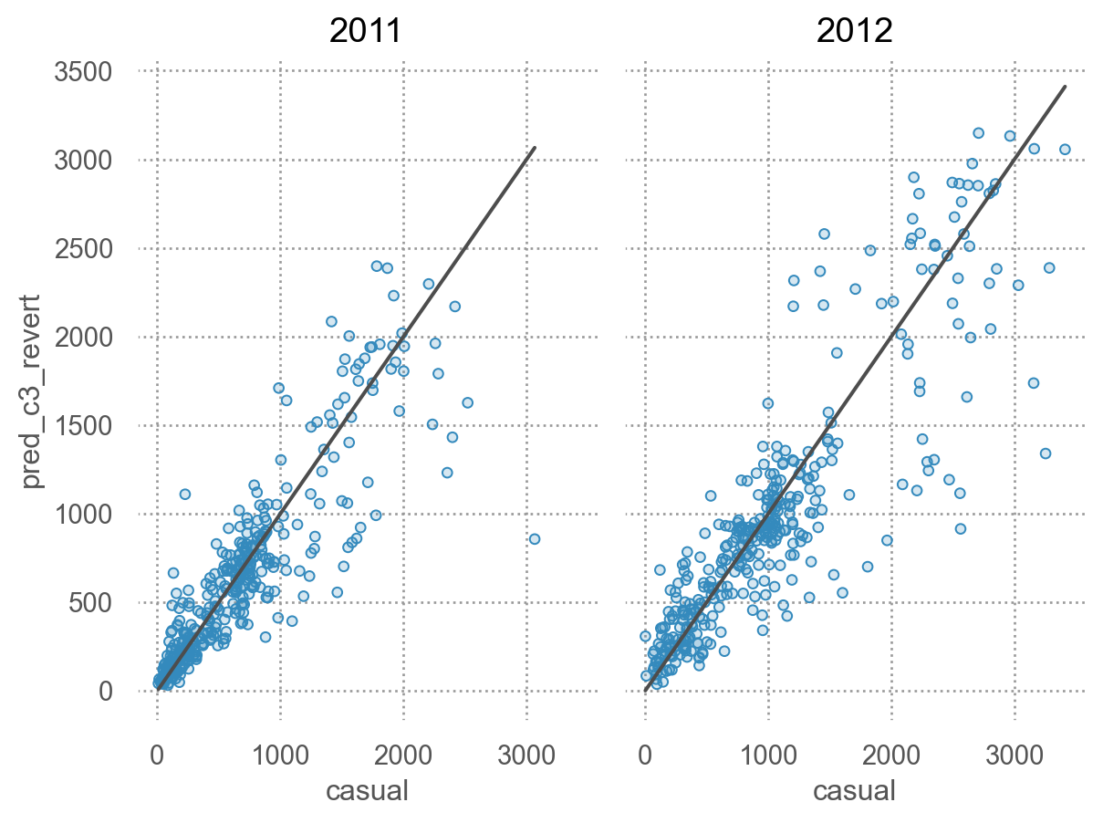
# 예측값과 실제값 비교 = 'casual' , y= 'pred_c3_revert' )= ".3" ), y= 'casual' )"year" )
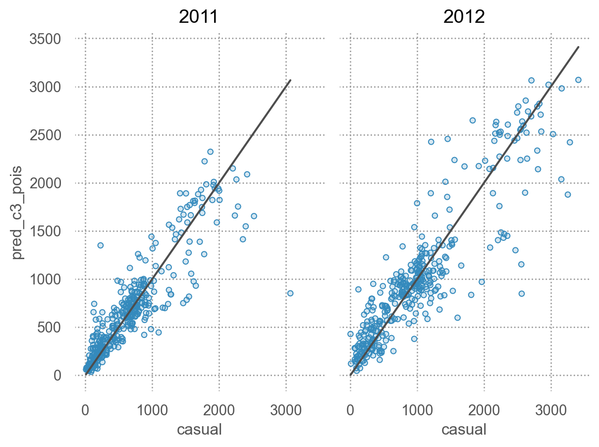
# 예측값과 실제값 비교: Poisson regression = 'casual' , y= 'pred_c3_pois' )= ".3" ), y= 'casual' )"year" )
모형의 비교와 각 예측변수의 공헌도
= smf.ols("lcasual ~ year" , data= bikes_daily).fit()= smf.ols("lcasual ~ year + temp + I(temp**2)" , data= bikes_daily).fit()= smf.ols("lcasual ~ year + temp + I(temp**2) + month" , data= bikes_daily= smf.ols("lcasual ~ year + temp + I(temp**2) + month + bs(hum, 4)" , data= bikes_daily= smf.ols("lcasual ~ year + temp + I(temp**2) + month + bs(hum, 4) + wday" , data= bikes_dailyprint (f" year: { mod_c_year. rsquared:.3f} \n " ,f"year + temperature: { mod_c_temp. rsquared:.3f} \n " ,f"year + temperature + months: { mod_c_month. rsquared:.3f} \n " ,f"year + temperature + months + humidity: { mod_c_hum. rsquared:.3f} \n " ,f"year + temperature + months + days of the week: { mod_c_wday. rsquared:.3f} " ,
 year: 0.057
 year + temperature: 0.554
 year + temperature + months: 0.588
 year + temperature + months + humidity: 0.660
 year + temperature + months + days of the week: 0.824
예측값을 original scale로 다시 되돌려 R squared 계산
R-squared with the original scale
= bikes_daily.assign(= lambda x: 2 ** mod_c_year.fittedvalues - 1 ,= lambda x: 2 ** mod_c_temp.fittedvalues - 1 ,= lambda x: 2 ** mod_c_month.fittedvalues - 1 ,= lambda x: 2 ** mod_c_hum.fittedvalues - 1 ,= lambda x: 2 ** mod_c_wday.fittedvalues - 1 ,from sklearn.metrics import r2_scorefor col in ["pred_c_year" , "pred_c_temp" , "pred_c_month" , "pred_c_hum" , "pred_c_wday" ]:= r2_score(bikes_daily_resid2["casual" ], bikes_daily_resid2[col])print (f" { col} : { r2:.2f} " )
pred_c_year: -0.08
pred_c_temp: 0.34
pred_c_month: 0.37
pred_c_hum: 0.42
pred_c_wday: 0.80
포아송 회귀 로 살펴보면,
X의 값에 따라 Y의 분포가 달라지는 경우, R-squared는 의미가 없음
데이터를 train/test로 나누어 평가하는 것이 더 적절함
= smf.poisson("casual ~ (temp + I(temp**2)) + year + wday" , data= bikes_daily).fit()= smf.poisson("casual ~ year" , data= bikes_daily).fit()= smf.poisson("casual ~ year + temp + I(temp**2)" , data= bikes_daily).fit()= smf.poisson("casual ~ year + temp + I(temp**2) + month" , data= bikes_daily= smf.ols("lcasual ~ year + temp + I(temp**2) + month + bs(hum, 4)" , data= bikes_daily= smf.poisson("casual ~ year + temp + I(temp**2) + month + bs(hum, 4) + wday" , data= bikes_dailyprint (f" year: { mod_c_pois_year. prsquared:.3f} \n " , # prsquared: pseudo R-squared f"year + temperature: { mod_c_pois_temp. prsquared:.3f} \n " ,f"year + temperature + months: { mod_c_pois_month. prsquared:.3f} \n " ,f"year + temperature + months + humidity: { mod_c_pois_hum. rsquared:.3f} \n " ,f"year + temperature + months + days of the week: { mod_c_pois_wday. prsquared:.3f} " ,
Optimization terminated successfully.
         Current function value: 60.868155
         Iterations 7
Optimization terminated successfully.
         Current function value: 245.676778
         Iterations 5
Optimization terminated successfully.
         Current function value: 140.141516
         Iterations 6
Optimization terminated successfully.
         Current function value: 130.926793
         Iterations 7
Optimization terminated successfully.
         Current function value: 43.674208
         Iterations 7
 year: 0.066
 year + temperature: 0.467
 year + temperature + months: 0.502
 year + temperature + months + humidity: 0.660
 year + temperature + months + days of the week: 0.834