Modelling Building 1 Exercises

R for Data Science by Wickham & Grolemund

# numerical calculation & data frames
import numpy as np
import pandas as pd

# visualization
import matplotlib.pyplot as plt
import seaborn as sns
import seaborn.objects as so

# statistics
import statsmodels.api as sm

# pandas options
pd.set_option('mode.copy_on_write', True)  # pandas 2.0
pd.options.display.float_format = '{:.2f}'.format  # pd.reset_option('display.float_format')
pd.options.display.max_rows = 7  # max number of rows to display

# NumPy options
np.set_printoptions(precision = 2, suppress=True)  # suppress scientific notation

# For high resolution display
import matplotlib_inline
matplotlib_inline.backend_inline.set_matplotlib_formats("retina")

Flights to SFO

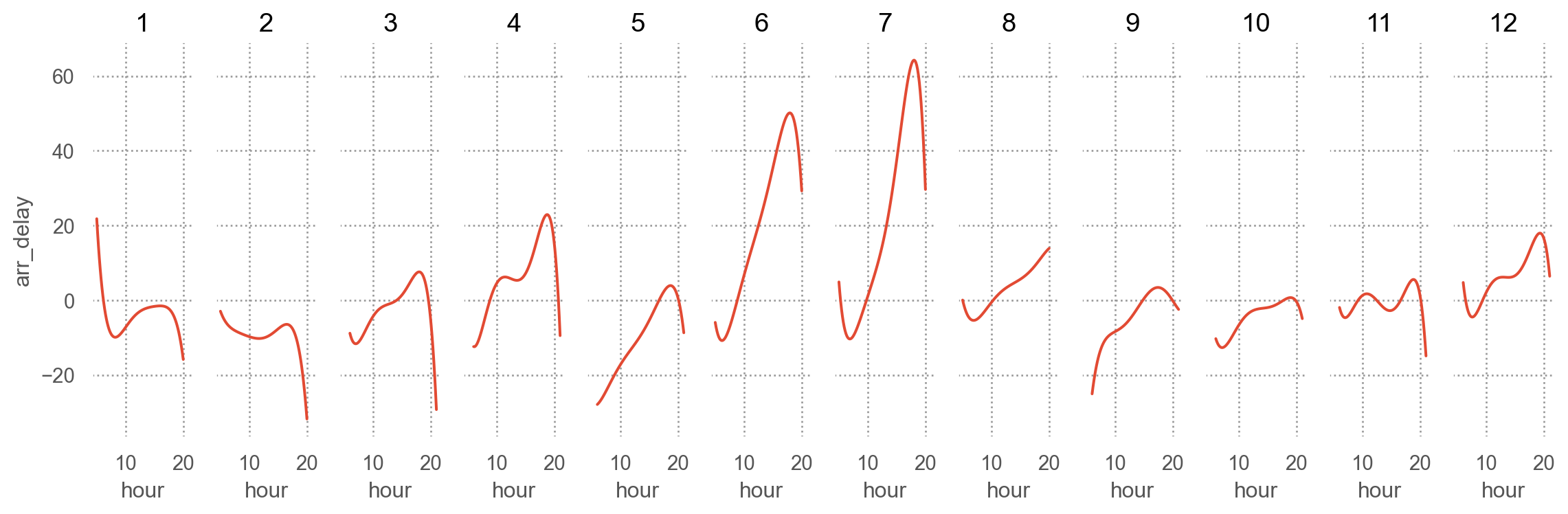
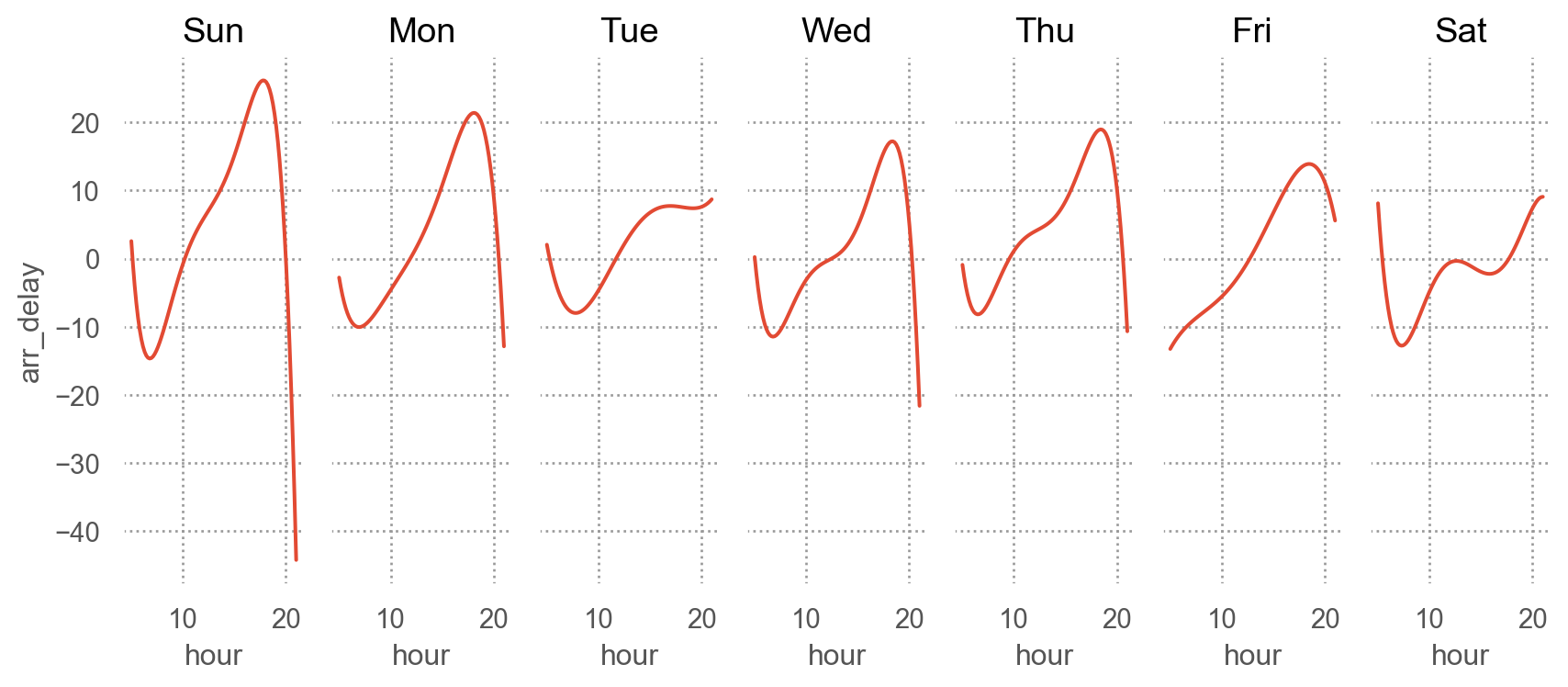
# import the data
flights = sm.datasets.get_rdataset('flights', 'nycflights13').data

# convert the date column to a datetime object
flights["time_hour"] = pd.to_datetime(flights["time_hour"])

# add a column for the day of the week
flights["dow"] = (
    flights["time_hour"]
    .dt.day_name()
    .str[:3]
    .astype("category")
    .cat.set_categories(["Sun", "Mon", "Tue", "Wed", "Thu", "Fri", "Sat"])
)

# add a column for the season
flights["season"] = np.where(flights["month"].isin([6, 7]), "summer", "other month")

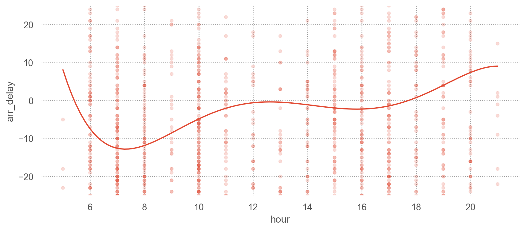
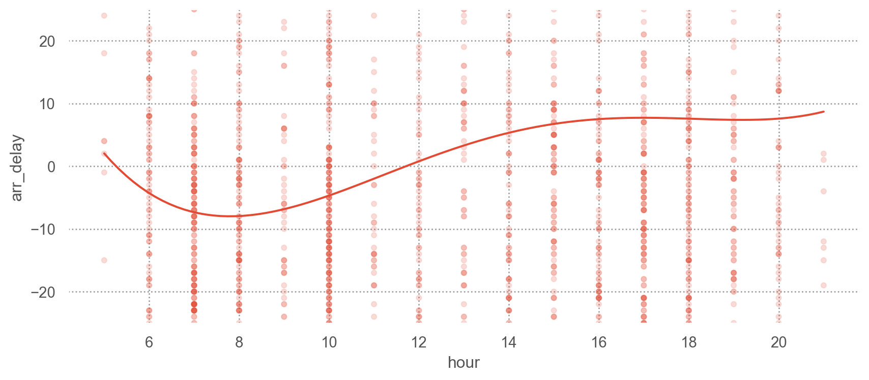
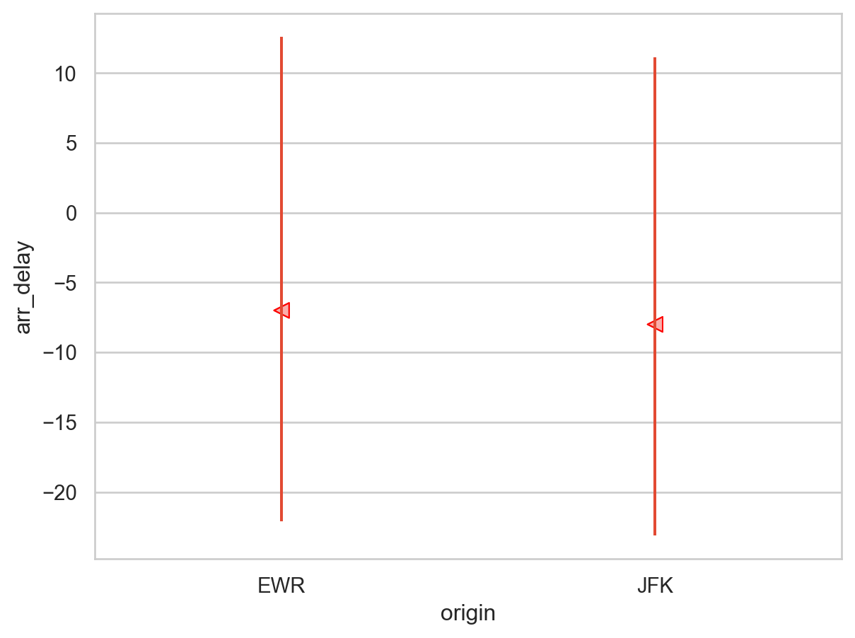
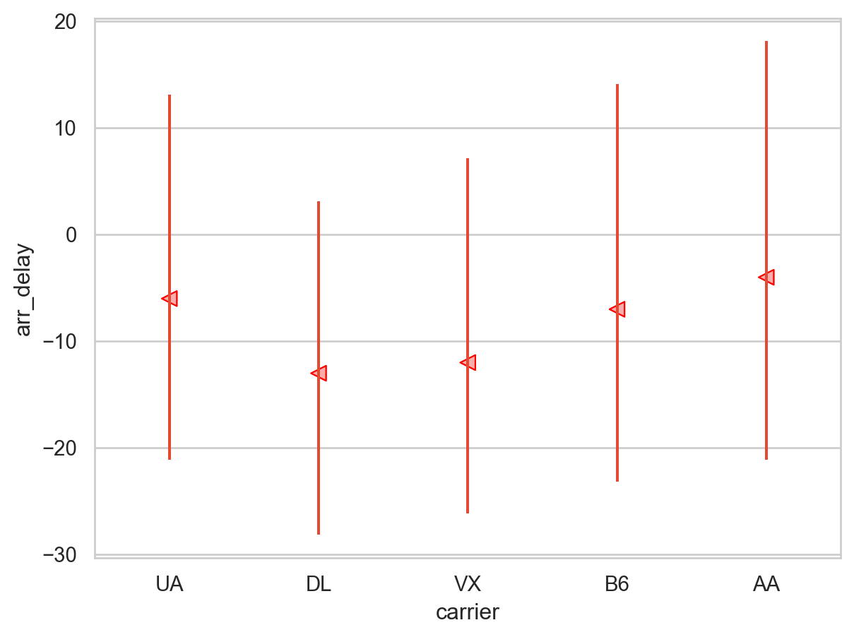
# filter out the flights to SFO
sfo = flights.query('dest == "SFO" & arr_delay < 500').copy()

from statsmodels.formula.api import ols
mod = ols("arr_delay ~ hour + origin + carrier + season + dow", data=sfo).fit()

이미 세운 모형의 잔차를 분석

sfo["resid"] = mod.resid

(
    so.Plot(sfo, x='hour', y='resid')
    #.add(so.Dots(alpha=.1))
    .add(so.Line(), so.PolyFit(5))
)

(
    so.Plot(sfo, x='hour', y='resid')
    .add(so.Line(), so.PolyFit(5))
    .facet("season")
)

(
    so.Plot(sfo, x='hour', y='resid')
    .add(so.Line(), so.PolyFit(5))
    .facet(row="season", col="dow")
    .layout(size=(9, 6))
)

처음부터 변수들 간의 관계를 파악하면서 모형을 세운다면,

(
    so.Plot(sfo, x='hour', y='arr_delay')
    #.add(so.Dots(alpha=.1))
    .add(so.Line(), so.PolyFit(5))
)

(
    so.Plot(sfo, x='hour', y='arr_delay')
    #.add(so.Dots(alpha=.1))
    .add(so.Line(), so.PolyFit(5))
    .facet("month")
    .layout(size=(12, 4))
)

(
    so.Plot(sfo, x='hour', y='arr_delay')
    #.add(so.Dots(alpha=.1))
    .add(so.Line(), so.PolyFit(5))
    .facet("dow")
    .layout(size=(9, 4))
)

(
    so.Plot(sfo.query('dow == "Sat"'), x='hour', y='arr_delay')
    .add(so.Dots(alpha=.1))
    .add(so.Line(), so.PolyFit(5))
    .layout(size=(9, 4))
    .limit(y=(-25, 25))
)

(
    so.Plot(sfo.query('dow == "Tue"'), x='hour', y='arr_delay')
    .add(so.Dots(alpha=.1))
    .add(so.Line(), so.PolyFit(5))
    .layout(size=(9, 4))
    .limit(y=(-25, 25))
)

from sbcustom import rangeplot
rangeplot(sfo, x='origin', y='arr_delay')

rangeplot(sfo, x='carrier', y='arr_delay')

print(mod.summary(slim=True))

                            OLS Regression Results                            
==============================================================================
Dep. Variable:              arr_delay   R-squared:                       0.096
Model:                            OLS   Adj. R-squared:                  0.095
No. Observations:               13169   F-statistic:                     107.0
Covariance Type:            nonrobust   Prob (F-statistic):          8.13e-275
====================================================================================
                       coef    std err          t      P>|t|      [0.025      0.975]
------------------------------------------------------------------------------------
Intercept          -20.4363      2.116     -9.660      0.000     -24.583     -16.289
origin[T.JFK]        4.1590      0.966      4.306      0.000       2.266       6.052
carrier[T.B6]       -9.5832      1.807     -5.302      0.000     -13.126      -6.040
carrier[T.DL]      -17.9685      1.553    -11.571      0.000     -21.012     -14.925
carrier[T.UA]       -4.0238      1.424     -2.826      0.005      -6.815      -1.232
carrier[T.VX]       -4.9082      1.537     -3.194      0.001      -7.921      -1.896
season[T.summer]    24.6238      0.991     24.838      0.000      22.681      26.567
dow[T.Mon]          -2.6982      1.424     -1.895      0.058      -5.489       0.093
dow[T.Tue]          -6.0939      1.423     -4.282      0.000      -8.883      -3.304
dow[T.Wed]          -5.3144      1.425     -3.728      0.000      -8.108      -2.520
dow[T.Thu]          -1.2890      1.425     -0.905      0.366      -4.082       1.504
dow[T.Fri]          -4.9515      1.422     -3.483      0.000      -7.738      -2.165
dow[T.Sat]         -10.3953      1.518     -6.847      0.000     -13.371      -7.419
hour                 2.0666      0.086     23.944      0.000       1.897       2.236
====================================================================================

Notes:
[1] Standard Errors assume that the covariance matrix of the errors is correctly specified.

mod = ols("arr_delay ~ hour + origin + carrier + season + dow", data=sfo).fit()

# origin removed
mod1 = ols("arr_delay ~ hour + carrier + season + dow", data=sfo).fit()

# carrier removed
mod2 = ols("arr_delay ~ hour + season + dow", data=sfo).fit()

print(f"R-squared: {mod.rsquared:.3f}, {mod1.rsquared:.3f}, {mod2.rsquared:.3f}")

R-squared: 0.096, 0.094, 0.084

# hour와 season이 상호작용하는 것으로 가정
mod3 = ols("arr_delay ~ hour * season + origin + carrier + dow", data=sfo).fit()

# hour와 모든 달과 상호작용하는 것으로 가정
mod4 = ols("arr_delay ~ hour * C(month) + origin + carrier + dow", data=sfo).fit()  # C(month) : month를 범주형 변수로 취급

# hour, 모든 달, 요일이 서로 상호작용하는 것으로 가정
mod5 = ols("arr_delay ~ hour * C(month) * dow + origin + carrier", data=sfo).fit()  # C(month) : month를 범주형 변수로 취급

print(f"R-squared: {mod.rsquared:.3f}, {mod3.rsquared:.3f}, {mod4.rsquared:.3f}, {mod5.rsquared:.3f}")

R-squared: 0.096, 0.118, 0.136, 0.177

Sample에서 더 많은 변량이 설명된다는 것이 반드시 좋은 모형을 의미하지는 않음!
통계에서는 adjusted(shrunken) R-squared로 보정

print(mod5.summary().tables[0])

                            OLS Regression Results                            
==============================================================================
Dep. Variable:              arr_delay   R-squared:                       0.177
Model:                            OLS   Adj. R-squared:                  0.166
Method:                 Least Squares   F-statistic:                     16.25
Date:                Tue, 03 Dec 2024   Prob (F-statistic):               0.00
Time:                        03:09:23   Log-Likelihood:                -67798.
No. Observations:               13169   AIC:                         1.359e+05
Df Residuals:                   12996   BIC:                         1.372e+05
Df Model:                         172                                         
Covariance Type:            nonrobust                                         
==============================================================================

Cross-validation
5-fold cross-validation을 통해 모형의 성능을 평가

from sklearn.model_selection import KFold
from sklearn.model_selection import cross_val_score
from sklearn.metrics import root_mean_squared_error, r2_score, mean_absolute_error


def cv_score(mod):
    print(f"the number of parameters: {mod.df_model}\n")

    kfold = KFold(5, shuffle=True, random_state=0)
    ave_r2, ave_aic, ave_bic = 0, 0, 0

    for i, (train_idx, test_idx) in enumerate(kfold.split(sfo)):
        sfo_train, sfo_test = sfo.iloc[train_idx], sfo.iloc[test_idx]
        
        mod_ = ols(mod.model.formula, data=sfo_train).fit()

        # R-squared
        r2_train = r2_score(sfo_train["arr_delay"], mod_.predict(sfo_train))
        r2_test = r2_score(sfo_test["arr_delay"], mod_.predict(sfo_test))
        ave_r2 += r2_test

        # AIC, BIC
        aic, bic = mod_.aic, mod_.bic
        ave_aic += aic
        ave_bic += bic

        print(f"Fold {i+1}: Train R2: {r2_train:.2f}, Test R2: {r2_test:.2f}")

    print(f"\nAverage Test R2: {ave_r2/5:.2f}")
    print(f"Average AIC: {ave_aic/5:.2f}, Average BIC: {ave_bic/5:.2f}")

cv_score(mod5)

the number of parameters: 172.0

Fold 1: Train R2: 0.19, Test R2: 0.12
Fold 2: Train R2: 0.18, Test R2: 0.13
Fold 3: Train R2: 0.18, Test R2: 0.17
Fold 4: Train R2: 0.17, Test R2: 0.18
Fold 5: Train R2: 0.18, Test R2: 0.16

Average Test R2: 0.15
Average AIC: 108788.40, Average BIC: 110044.81

cv_score(mod4)

the number of parameters: 34.0

Fold 1: Train R2: 0.14, Test R2: 0.11
Fold 2: Train R2: 0.14, Test R2: 0.12
Fold 3: Train R2: 0.13, Test R2: 0.14
Fold 4: Train R2: 0.13, Test R2: 0.14
Fold 5: Train R2: 0.14, Test R2: 0.14

Average Test R2: 0.13
Average AIC: 109047.00, Average BIC: 109301.19

cv_score(mod3)

the number of parameters: 14.0

Fold 1: Train R2: 0.12, Test R2: 0.09
Fold 2: Train R2: 0.12, Test R2: 0.11
Fold 3: Train R2: 0.12, Test R2: 0.13
Fold 4: Train R2: 0.12, Test R2: 0.13
Fold 5: Train R2: 0.12, Test R2: 0.13

Average Test R2: 0.12
Average AIC: 109229.17, Average BIC: 109338.10

# Spline regression
mod5_spline = ols("arr_delay ~ cr(hour, df=5) * C(month) * dow + origin + carrier", data=sfo).fit()

cv_score(mod5_spline)

the number of parameters: 424.0

Fold 1: Train R2: 0.21, Test R2: 0.10
Fold 2: Train R2: 0.21, Test R2: 0.12
Fold 3: Train R2: 0.20, Test R2: 0.14
Fold 4: Train R2: 0.20, Test R2: 0.16
Fold 5: Train R2: 0.20, Test R2: 0.15

Average Test R2: 0.14
Average AIC: 108957.71, Average BIC: 112044.26

# Ridge regression with polynomial features
from sklearn.preprocessing import PolynomialFeatures
from sklearn.linear_model import RidgeCV
from sklearn.pipeline import make_pipeline

kfold = KFold(5, shuffle=True, random_state=0)
sfo["month"] = sfo["month"].astype("category")  # 범주형 변수로 변환

X = sfo[["hour", "origin", "carrier", "month", "dow"]]
X = pd.get_dummies(X, drop_first=True)
y = sfo["arr_delay"]

poly = PolynomialFeatures(2)  # 모든 2차 항을 포함
ridge = RidgeCV()

pipe = make_pipeline(poly, ridge)
cross_val_score(pipe, X, y, cv=kfold, scoring="r2")

array([0.13, 0.15, 0.17, 0.19, 0.16])

# the number of parameters
poly.fit_transform(X).shape

(13169, 300)

# XGBoost
from xgboost import XGBRegressor

xgb = XGBRegressor(n_estimators=5000, learning_rate=0.01, max_depth=3, random_state=0)
cross_val_score(xgb, X, y, cv=kfold, scoring="r2")

array([0.13, 0.15, 0.18, 0.19, 0.18])